Interaction Diagram for Concrete Columns: Comparing ACI 318-19 and AS 3600 Approaches

What is an interaction diagram?

An interaction diagram is a graphical representation of the ultimate strength of a concrete’s cross-section that is subject to combined axial and bending forces, such as a column. The analysis of how columns respond to these combined axial load (P) and bending moments (M) is known as column P M interaction.

‍

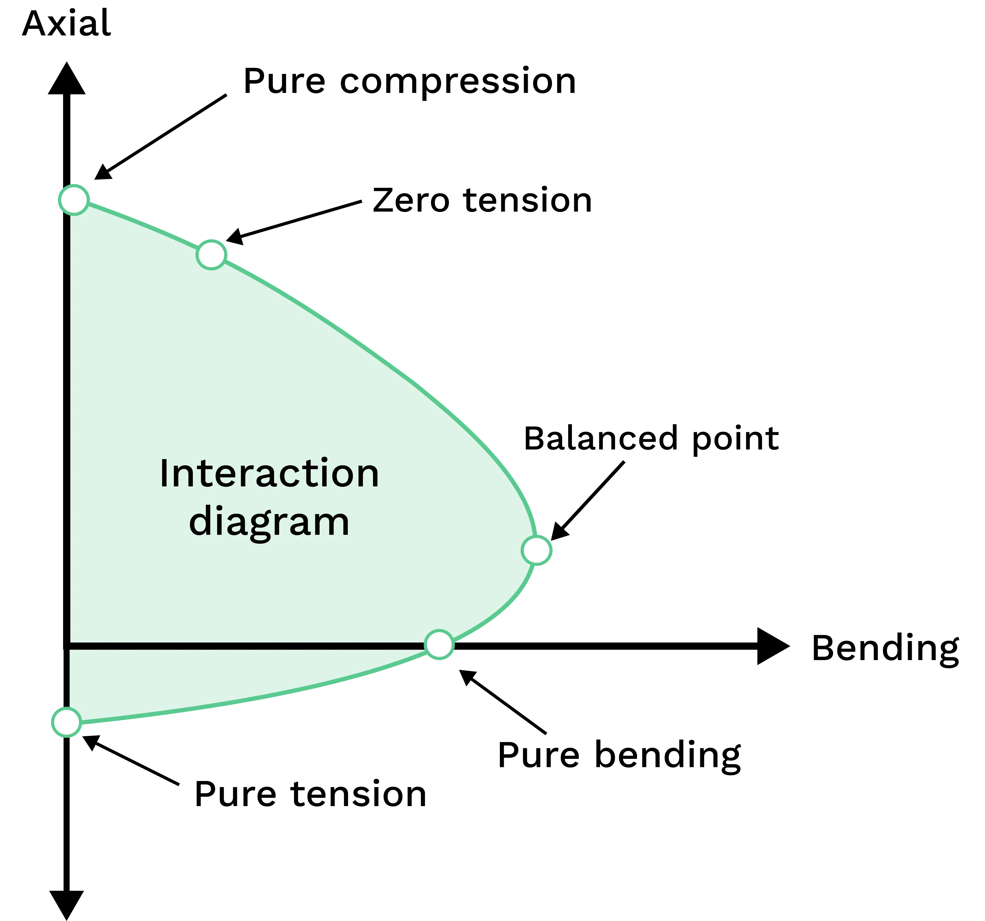
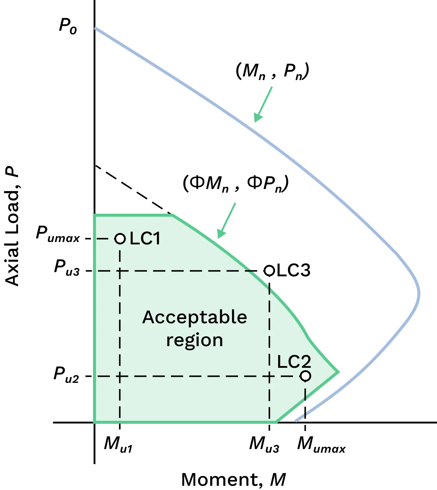
If the design axial and bending forces are within the region bound by the interaction diagram, then the concrete section is deemed to be safe as a structural member within a building framework.

Note, different parts of the world tend to have slightly different terminology. Australian’s call it an interaction diagram, Europeans call it a column chart while the Americans call it a P-M diagram. Australian’s and Europeans refer to axial load as N and bending with M while the American’s refer to axial load as \(P\).

The term 'column section' refers to the cross-sectional area being analyzed in the interaction diagram.

1. Fundamental assumptions

The construction of the interaction diagram is based on the applicable conditions of equilibrium and strain compatibility, which are essential for accurate analysis of reinforced concrete columns.

The fundamental assumptions to construct the interaction diagram are:

• Equilibrium and strain compatibility: These two principles ensure accurate analysis of reinforced concrete columns. Force equilibrium requires that internal forces balance external loads, while strain compatibility means embedded steel deforms consistently with the surrounding concrete. Together, they form the basis for strength design in accordance with code requirements.
• Plane sections remain plane: cross-section that was a flat plane before bending will remain a flat plane after bending
• Zero concrete tensile capacity: concrete exhibits negligible resistance to tensile loads.
• The compressive stress distribution in concrete is often simplified using an equivalent rectangular stress block, as defined by the rectangular stress block CSA (CSA A23.3-94). The depth of the equivalent rectangular stress block is a key parameter in this simplification.

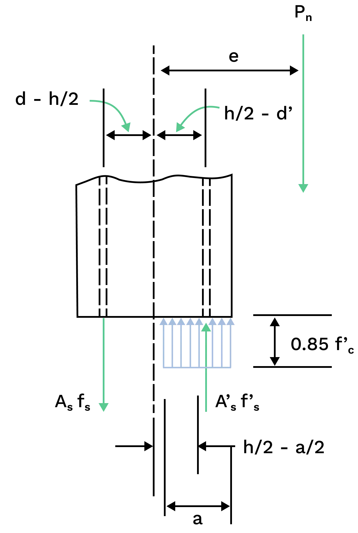
1.1 Force equilibrium

The interaction diagram represents this equilibrium by illustrating the axial load and bending moment combinations a column can safely resist. Each point reflects a balanced state of internal forces. As loading increases, stress distribution shifts, reducing the column’s resistance. Both internal forces and their lever arms are considered to assess column behaviour under combined actions. The analysis of forces and moment arms is essential in establishing equilibrium, as it determines how the internal actions balance the applied loads.

1.2 Strain compatibility

Strain compatibility ensures that deformations in concrete and steel follow the section’s geometry. This principle ensures stresses are properly distributed, allowing concrete and reinforcement to work together under load. Concrete typically undergoes compressive strain, while steel may experience tension or compression depending on the loading.

Under bending, the strain distribution across the section remains linear. The neutral axis depth and strain profile are measured from the compression edge. The distance from the extreme compression fiber to the neutral axis is a critical parameter in strain compatibility analysis, as it directly affects the calculation of strains and stresses in reinforced concrete elements.

Mathematically, strain compatibility relates concrete and steel strain through the section’s geometry and Hooke’s Law.

Geometrically:

$$ϵ_s=ϵ_u(d−c_c)$$ $$ϵ_s′=ϵ_u(c−d’_c)$$

Hooke’s Law:

$$f_s=E_sϵ_s$$ $$f’_s=E_sϵ’_s$$

Where:

\(E_s\): Modulus of Elasticity of the reinforcing steel.

2. Design Steps

2.1 Axial Compression Strength

The relationship between axial load strength and the P-M diagram is rooted in how columns resist combined forces. In pure compression (no moment), the axial load capacity represents the maximum compressive strength before failure, calculated as the sum of concrete and steel compressive contributions, adjusted by safety factors.

When bending is introduced, part of the section must resist additional stresses, reducing its axial capacity. The stress distribution changes from uniform (in pure compression) to a linear gradient—compression on one side, tension on the other.

This interaction produces the curved boundary of the P-M diagram, showing the limit combinations of axial load and moment. For normal-strength concrete, compressive strength is typically reduced to \(0.85f’_c\) in design.

The ultimate axial strength of the element is attained when the concrete undergoes crushing failure, and the reinforcement steel yields:

$$P_n=0.85f’_c(A_g−A_s)+f_yA_s$$

In this formula, the area of the reinforcement ($A_s$) is included in the calculation of the total compressive force, ensuring that both the concrete and the reinforcement contributions are properly accounted for. The area of reinforcement is included in the area used to compute the total compressive strength, so the included area directly affects the value used to compute the axial load capacity.

Where:

\(f’_c\) = (Compressive Strength of Concrete):

Compressive strength of concrete. It measures the maximum compressive stress that concrete can withstand under axial loads.

\(A_g\) = (Gross Sectional Area):

Total cross-sectional area of a structural element, such as a column or a beam. It includes the area of both the concrete and any reinforcing steel.

\(f_y\) = (Steel Yield Stress):

Yield strength of the reinforcing steel. It indicates the stress at which the steel exhibits significant plastic deformation.

\(A_s\) = (Total Longitudinal Reinforcement Area):

The total cross-sectional area of a concrete element’s longitudinal (primary) reinforcement. It is the sum of the cross-sectional areas of all the individual longitudinal bars.

2.2 Axial Tensile Strength

The concrete is fully fissured when the ultimate axial tensile strength is reached, rendering its contribution null. Therefore, the ultimate strength is attained when the reinforcement reaches its yield stress. In this case, the capacity is governed by the tension steel, which yields as the concrete cracks completely at the tension face of member.

$$P_{nt}=f_yA_s$$

In the tension-controlled region of the P-M diagram, capacity is limited to the steel’s yield strength. The tension face becomes critical as reinforcement yields and concrete no longer carries tension.

This region shows significantly lower capacity compared to compression-controlled zones. The point of maximum tension on the P-M diagram corresponds to the greatest tensile force the section can resist under combined axial and bending loads. The P-M diagram serves as a key tool to visualise safe axial and bending load combinations while accounting for material properties and section geometry.

Other influencing factors include:

• Material Strengths: Higher concrete and steel strengths raise capacity.
• Reinforcement Ratio: Higher ratios can improve strength but may reduce ductility.
• Slenderness: Slender columns are prone to buckling, which reduces effective axial capacity and shifts the interaction curve downward.

By understanding these relationships, engineers can use the P-M diagram to ensure safe and efficient column design under complex loading conditions.

2.3 Balanced Failure of Strains

Balanced failure in flexo-compression refers to the condition where concrete in compression and tensile reinforcement both reach their respective limit states at the same time. This marks the transition between compression- and tension-controlled behaviour. This transition is defined by the compression controlled strain limit, which distinguishes the strain distribution at which the section shifts from compression failure modes to tension failure initiated by reinforcement yield.

According to ACI, the maximum compressive strain for concrete is typically taken as 0.003. At this balanced point, both materials are fully utilised, achieving an efficient design that leverages the strength of both concrete and steel.

$$c = c_b =  \frac{dϵ_u}{ϵ_u + ϵy}$$

3. How to generate the interaction diagram

Keeping the above assumptions in mind, interaction diagrams can be generated by analysing the reinforced concrete section under combined axial and bending loads. For a tied reinforced concrete column, a diagram tied reinforced concrete is generated, and the interaction diagram tied reinforced illustrates the load and moment capacity for such columns.

The curve is defined by a set of key limit states:

• Pure Compression: Maximum axial load with zero moment.
• Balanced Failure: Concrete and reinforcement reach ultimate strains simultaneously.
• Compression-Controlled: Concrete crushes before the steel yields.
• Pure Moment: Pure bending without axial load ().
• Pure Axial Tension: Reinforcement yields after the concrete cracks completely under tension.

Each of these points defines the boundary of the interaction diagram and represents a unique strain and force distribution across the section. The maximum tensile capacity is governed entirely by the yield strength of the reinforcement, represented by the pure axial tension point on the diagram.

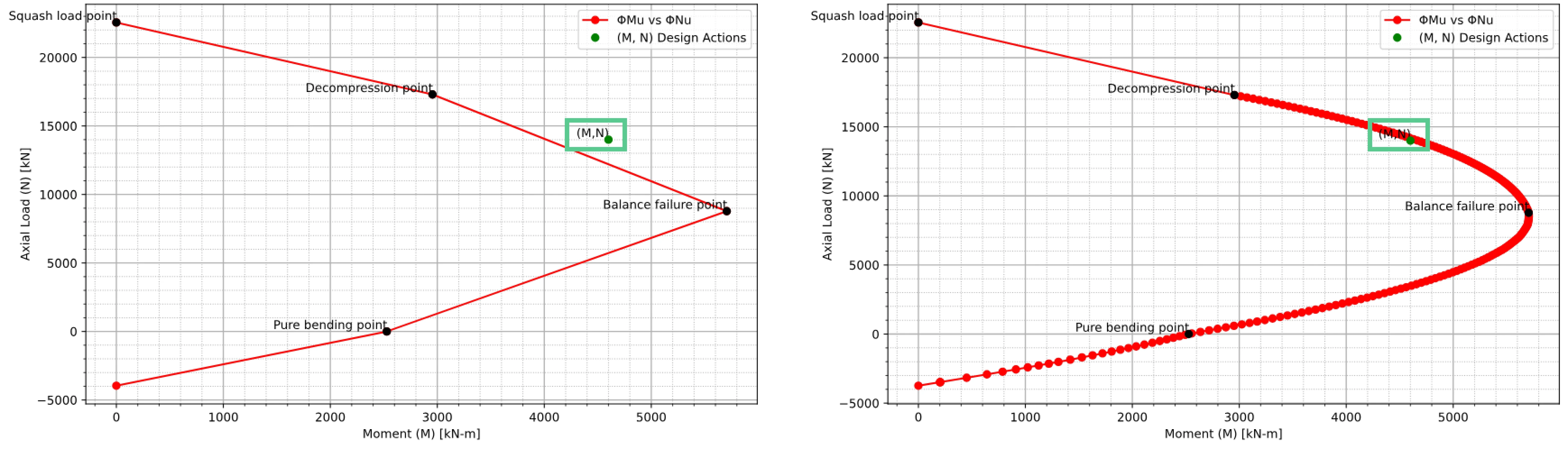
3.1 By hand

Manually, we determine the coordinates of each key point and draw a best-fit curve to visualise the safe design region. These points are plotted as (M, P) pairs for a given reinforcement layout and a specific neutral axis depth:

• Pure Compression (Squash Load): Failure under axial compression only.
• Decompression Point: Section loses tensile capacity under bending and compression.
• Balanced Point: Simultaneous concrete crushing and steel yielding.
• Pure Bending: Failure due to moment only.
• Pure Tension: Failure under tensile load as reinforcement yields.

At each point, stress and strain conditions define the failure mode, such as zero stress at the tension face or yielding at the compression face. Bar stress near tension and stress near tension face are critical parameters in these calculations, and values at the face of member equal to specific strain or stress levels are used to define control points on the interaction diagram. This method is conservative and can underestimate capacity compared to more refined approaches.

The depth of the neutral axis takes different symbols in the national codes. AS3600 takes \(k_ud\), EC2 takes X and ACI 318 takes c.

3.2 Using the computer

Modern structural engineering software generates interaction diagrams using a high number of neutral axis positions, resulting in a smooth, curved diagram. Tools like spSection allow for precise modelling of reinforcement and irregular geometries. Program shortcuts and the spSection figure can be used to efficiently define the column section and reinforcement layout.

The general process is:

• Define a range of neutral axis depths \(k_ud\) from near zero to full section depth.
• For each :
  • The reinforcement in this layer is included in the force calculations, and as a result it is necessary to adjust the computed values accordingly.
  • Calculate strain in each bar using linear distribution.
  • Compute corresponding stress and axial force in each bar.
  • Determine concrete compression force using a rectangular stress block.
  • Sum all internal forces and moments to get \(N_u\) and \(M_u\).
  • Plot the \(M_u,N_u\) points using a tool like Python’s matplotlib to form the interaction diagram.

In some cases, it is necessary to subtract specific quantities (such as \(\alpha_1\phi_cf'_c\)) from the reinforcement force calculations to ensure accuracy.

This numerical method provides more accurate results and better represents the actual capacity of reinforced concrete sections, especially for irregular geometries and reinforcement layouts. The software can analyze both directions simultaneously for biaxial bending scenarios.

3.3 Comparison

The manual approach provides a conservative estimate of capacity by connecting a small number of critical points. This is particularly relevant for reinforced concrete column cross sections, where maximum compression and the depth of the neutral axis (c is depth) are key parameters. In contrast, the computational approach calculates many (N, M) pairs for various neutral axis depths, resulting in a smooth and more accurate interaction curve.

An important observation is how these methods influence safety margins. In some cases, design actions that fall outside the conservative diagram may actually lie within the accurate, curved diagram—highlighting the benefit of computational tools.

Additionally, the shape of the interaction diagram varies between design codes. For example:

• ACI 318 (USA) introduces a noticeable kink near the balanced point and a horizontal segment between pure compression and decompression points.
• AS 3600 (Australia) produces a smoother diagram with a linear transition in the same region.

For Canadian codes, detailed calculation procedures reference a23.3 94 8.4.2, a23.3 94 8.4.3, a23.3 94 10.0, a23.3 94 10.1.3, a23.3 94 equation, a23.3 94 equation 10, csa a23.3 94 12.15, and csa a23.3 94 10.1.7, including how the neutral axis is measured and the importance of c is depth in stress analysis.

These differences stem largely from each code’s treatment of the capacity reduction factor (φ):

• ACI 318-19: φ varies based on whether a section is compression-controlled, tension-controlled, or in transition. These states are defined by comparing net tensile strain (εₜ) to yield strain (εₜₐ).
• AS 3600-2018: φ varies depending on the type of action (e.g., bending without axial force) and whether the section is compression- or tension-controlled.

Computational methods often use the method and unified design approach, ensuring all conditions of strength satisfying equilibrium and strain compatibility are met for reinforced concrete columns.

Unbalanced moments due to irregular loading or boundary conditions may also affect the shape and safety limits of the interaction curve, reinforcing the need for flexible analysis tools. For interaction diagrams, x axis uniaxial bending and the position where the tensile strain is equal to the yield are important considerations.

Understanding these distinctions is critical for ensuring both code compliance and structural reliability across different design standards. The extreme layer of reinforcement is a key factor in determining the failure mode and the shape of the interaction diagram.