
Wavelet analysis of terrain in Python: map hummocky landslide ground from a DEM with a 2D wavelet transform and read its diffusion age. Open a copy free.

Tell us what you need, or sign up and build it yourself in minutes.
Leave your email and we'll tell you when a template for it is ready:






No items found.
No items found.
About this Wavelet Analysis Example
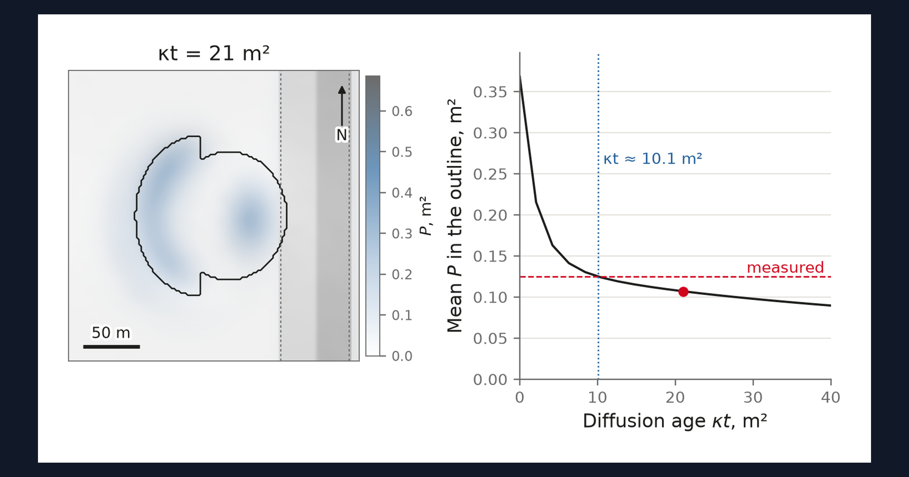
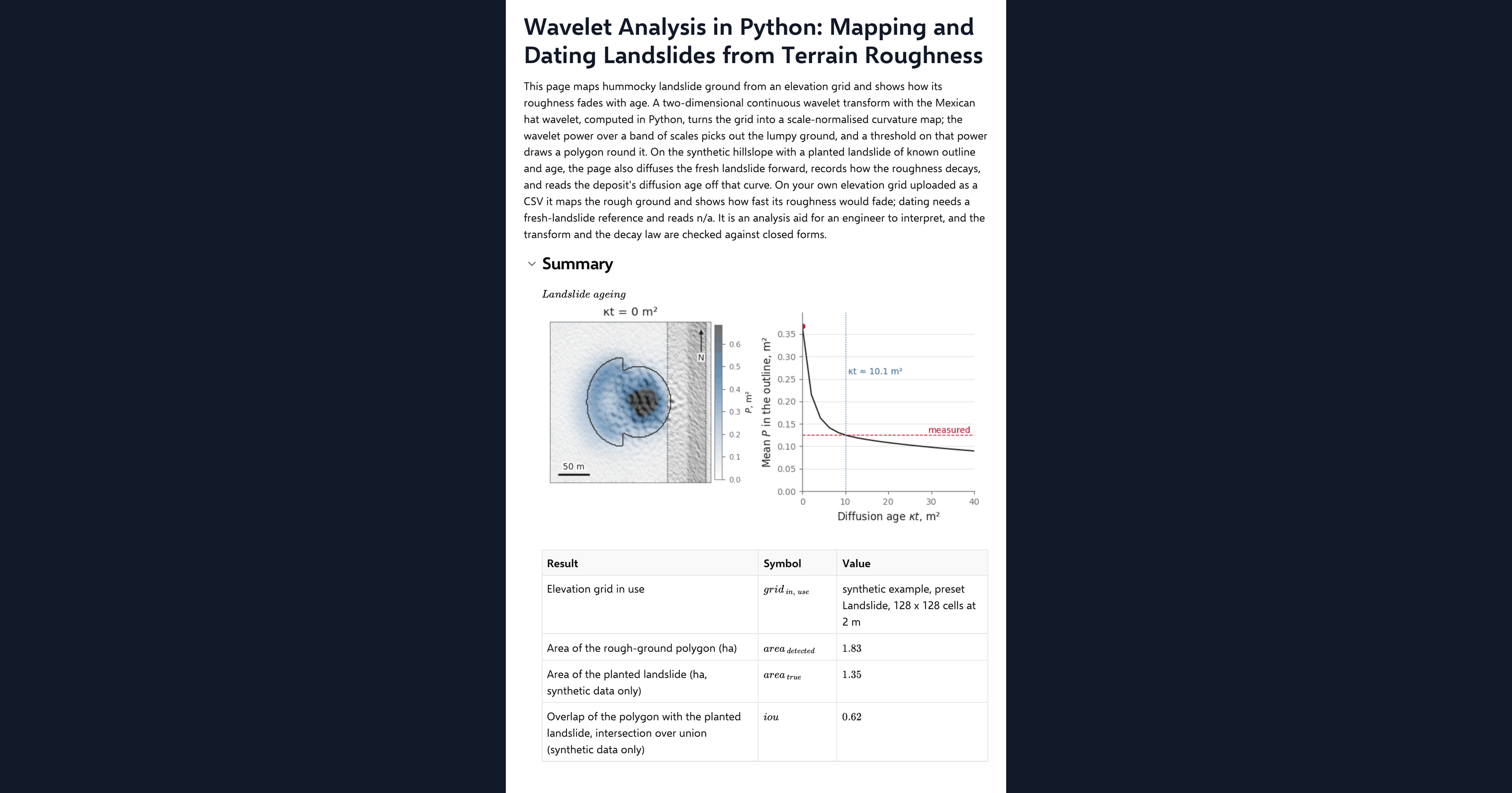
This page is a worked example of wavelet analysis of terrain in Python, inside a CalcTree calculation page. It maps hummocky landslide ground from an elevation grid and shows how its roughness fades with age. A two-dimensional continuous wavelet transform with the Mexican hat wavelet turns the grid into a scale-normalised curvature map; the wavelet power over a band of scales picks out the lumpy ground, and a threshold on that power draws a polygon round it. On the synthetic hillslope with a planted landslide of known outline and age, the page also diffuses the fresh landslide forward, records how its roughness decays and reads the deposit's diffusion age off that curve. It runs on your own elevation grid too.
- Engineering geologist or geotechnical engineer: map the hummocky ground on a slope from lidar, see which scales carry the signal, and get a relative age from the roughness in the way the published landslide inventories do.
- Engineer exploring Python in calculations: read a spectral wavelet transform, a polygon clean-up and a diffusion model in NumPy and SciPy on one page, with their closed-form checks.
- Graduate engineer learning terrain analysis: change the scales, the threshold and the age and watch the curvature map, the polygon and the decay curve respond.
It is an analysis aid, not a landslide assessment. It is an example of what a CalcTree page can do, built with CalcTree AI, not a design method to rely on as is. The model is idealised and its limits are stated on the page. Duplicate it into your own workspace to change the inputs, read the Python, or use it as the starting point for your own analysis, and verify anything you take into a real design.
More info on Wavelet Curvature
Inputs
A data source dropdown chooses the example terrain or your uploaded grid. For the example you set a terrain preset, grid resolution, the planted landslide and its diffusion age. The method inputs are the band of wavelet scales, the smoothing radius for the power map, the threshold factor over the background power, the channel buffer, the maximum age of the diffusion sweep and the hillslope diffusivity that turns a diffusion age into years. Your own elevation grid goes in as a CSV with x_m, y_m and z_m columns on a regular grid, loaded as a page dataset. The page refuses a grid that is not regular or is missing cells and says why, and it thins a grid wider than 192 cells a side to the smallest whole step that fits.
The wavelet transform
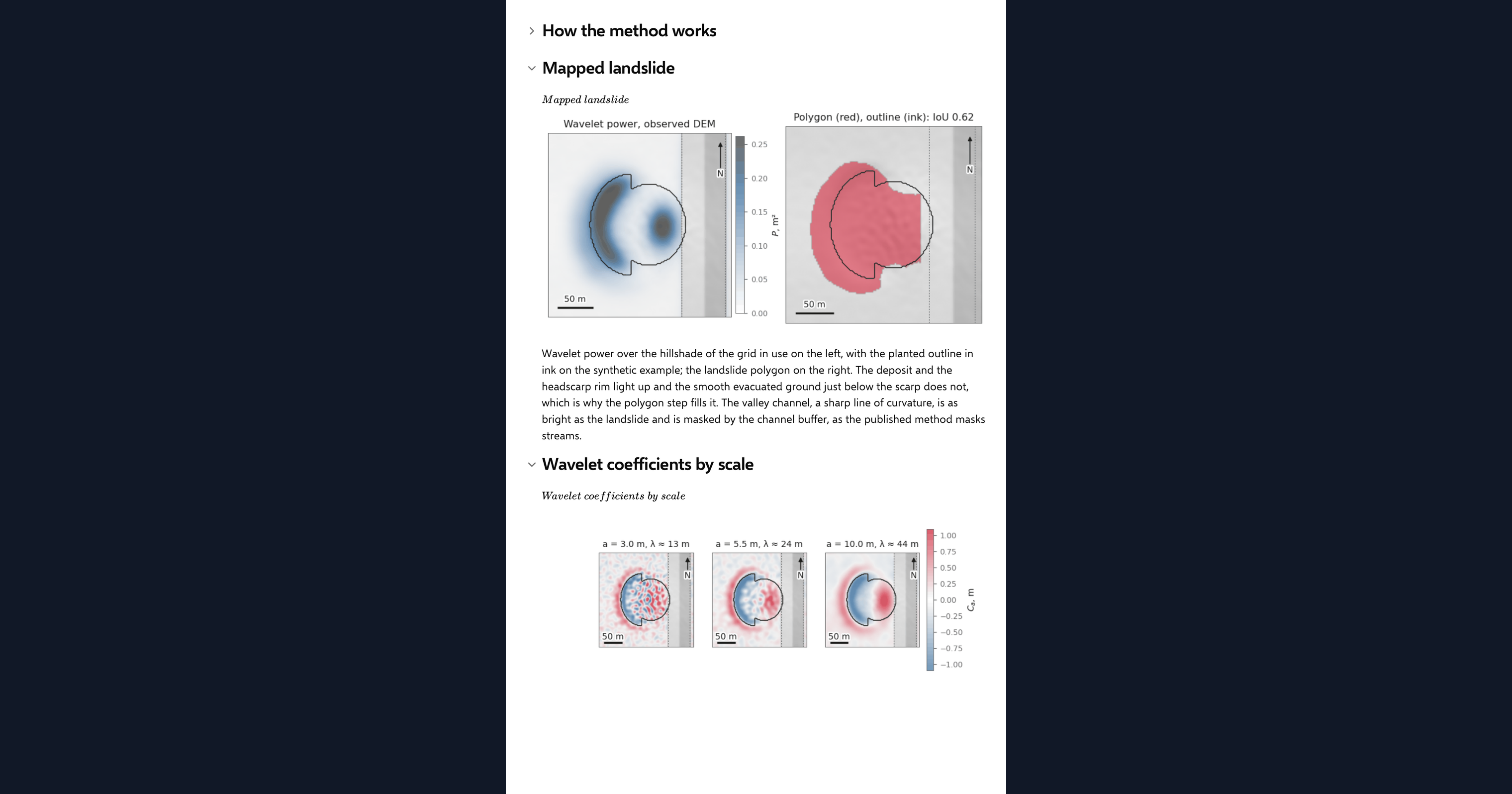
The Mexican hat wavelet is the negative Laplacian of a Gaussian, so convolving the grid with it at a scale gives the curvature of the surface smoothed to that scale, following Booth, Roering and Perron (2009). The page applies it in the Fourier domain on the plane-detrended grid with generous reflective padding, normalises by the square of the scale so that scales can be compared, and averages the squared coefficient over the band to get the wavelet power. Hummocky ground has high power at the scales of its hummocks; a smooth slope has almost none.
Mapping the landslide
Cells whose power exceeds a multiple of the median background power, outside the channel buffer, are closed, hole-filled and eroded by the smoothing radius to give the mapped polygon. On the example terrain the overlap with the planted outline and the mapped area against the true area are reported as results. The valley axis for the buffer is found as the strongest concave line across the site at the largest scale.
Dating by diffusion
A deposit smooths with time by hillslope diffusion, as described by Culling (1963), and its roughness at a given scale decays at a known rate. The page diffuses the fresh planted landslide forward over a range of diffusion ages, records the mean wavelet power inside the outline at each step, and reads the observed power off that curve to estimate the deposit's diffusion age, after Booth and others (2017) and LaHusen and others (2016). Divided by the diffusivity you enter, that is an age in years. On an uploaded grid there is no fresh reference, so the page diffuses your ground forward instead and reports the dating as n/a.
Checking the analysis
Three closed forms check the code: the wavelet coefficient at the crest of a Gaussian hill, the wavelet power of a sinusoid of known wavelength, and the decay of that power under diffusion. One agreement chip reports all three, with each error visible beside its tolerance.
Python libraries used
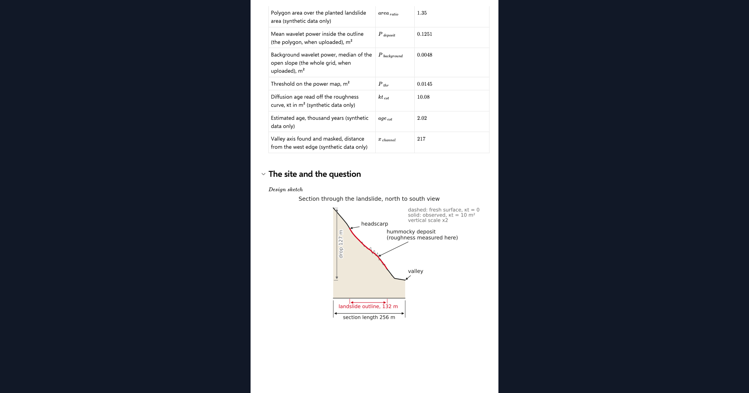
NumPy holds the grid and runs the Fourier transforms. SciPy cleans the polygon with binary morphology and smooths the power map. Matplotlib draws the hillshade, the curvature maps by scale, the mapped landslide, the decay curve, the ageing animation and the design sketch.
Common Calculation Errors to Avoid
- Padding only for the edge, not the wrap: a spectral convolution is periodic, and a detrended grid still jumps by the full plane drop across the FFT boundary. Detrend and pad by several times the largest scale, or bands appear along the edges.
- Comparing scales without normalising: the raw wavelet coefficient falls with scale even on a self-similar surface. Normalise by the square of the scale before comparing or averaging across the band.
- Thresholding without cleaning up: the rough ground sits on the scarp rim and the toe front, and smoothing dilates it. A raw threshold gives a ragged, oversized polygon; close, fill and erode it.
- Reading a gully as a landslide: gully heads carry wavelet power of their own and show as a false positive on a slide-free slope. Check any polygon against the hillshade.
- Treating the diffusion age as calendar years: the age in years depends on the diffusivity, which varies by an order of magnitude between climates and materials. Calibrate it for the site or report the diffusion age itself.
- Dating from an uploaded grid: without a fresh reference surface there is no decay curve to read against. The page diffuses your ground forward for comparison but will not report an age.
Engineering templates
Common calculators
Design guides




FAQs
Why use a wavelet rather than a simple roughness index?
A wavelet measures curvature at a chosen scale, so it can separate the hummocks of a landslide deposit from survey noise below them and from the hillside above them. A plain roughness index mixes all of those together.
What does the Mexican hat wavelet do?
It is the negative Laplacian of a Gaussian. Convolving the grid with it is the same as smoothing the surface to that scale and taking its curvature, which is why the maps look like curvature maps with the fine noise removed.
How does the page estimate the age of a landslide?
It diffuses the fresh planted landslide forward in time, records how the wavelet power inside the outline decays, and reads the observed power off that curve. The result is a diffusion age in square metres; dividing by the hillslope diffusivity gives years.
Can I map landslides on my own lidar data?
Yes. Upload a regular x_m, y_m, z_m grid as the page dataset and switch the data source. The curvature maps and the polygon then come from your ground, with no channel mask. Dating reads n/a because there is no fresh reference to diffuse.
How are the wavelet calculations checked?
Against three closed forms: the coefficient at the crest of a Gaussian hill, the power of a sinusoid at a known scale, and the decay of that power under diffusion. The page reports each error against its tolerance in one agreement chip.
Learn about the benefits of using CalcTree on engineering projects!