Topographic Position Index in Python: Ridge, Slope and Valley Mapping

About this Topographic Position Index Example

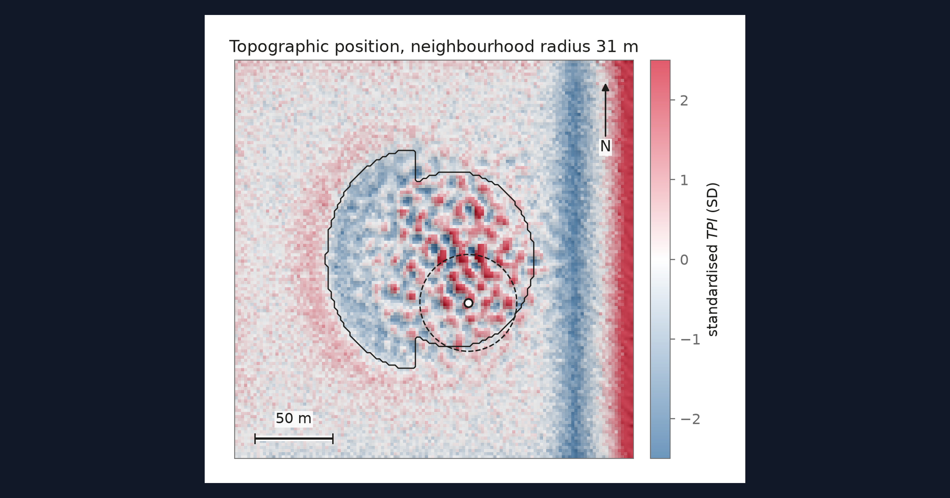
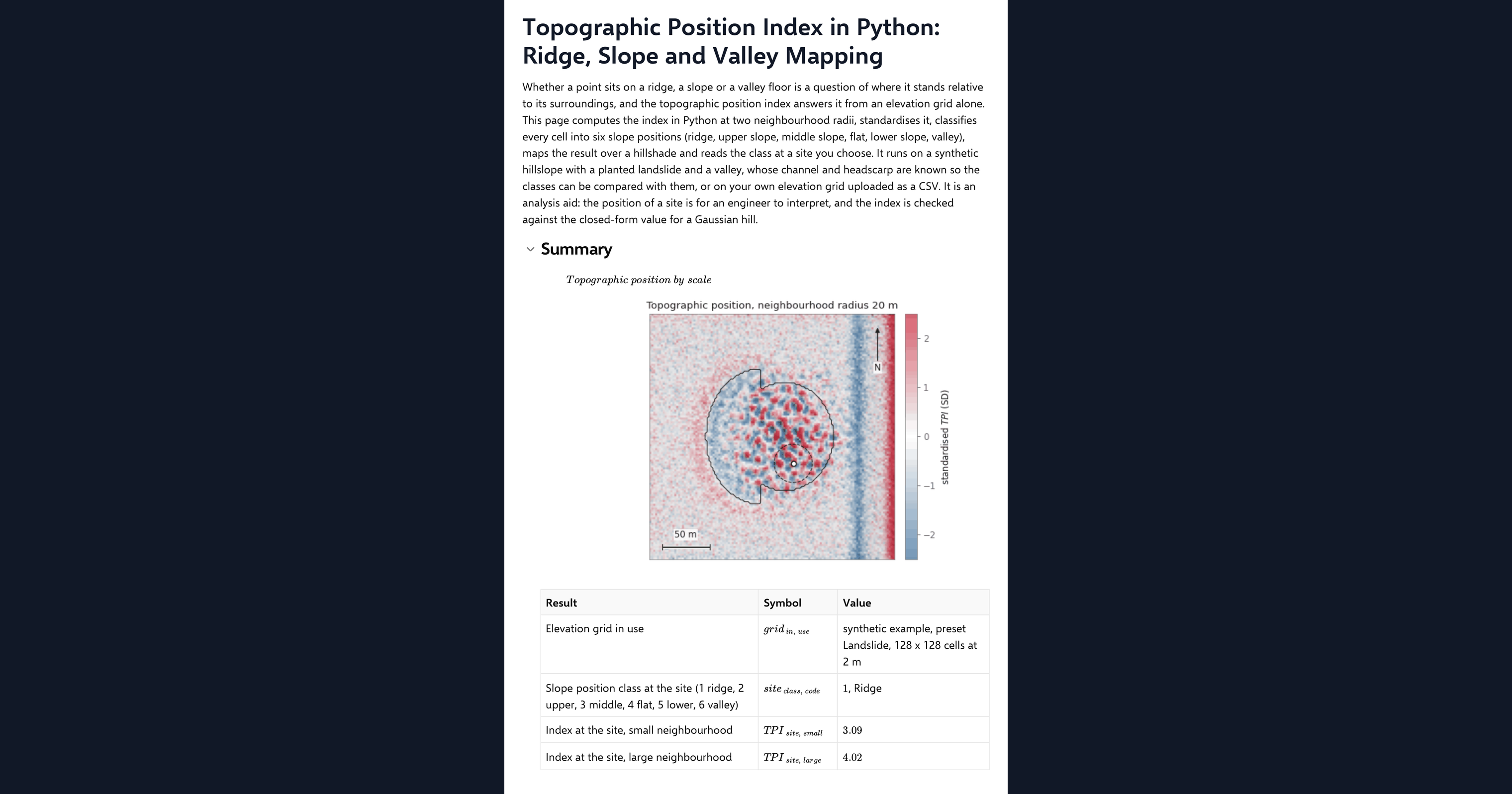
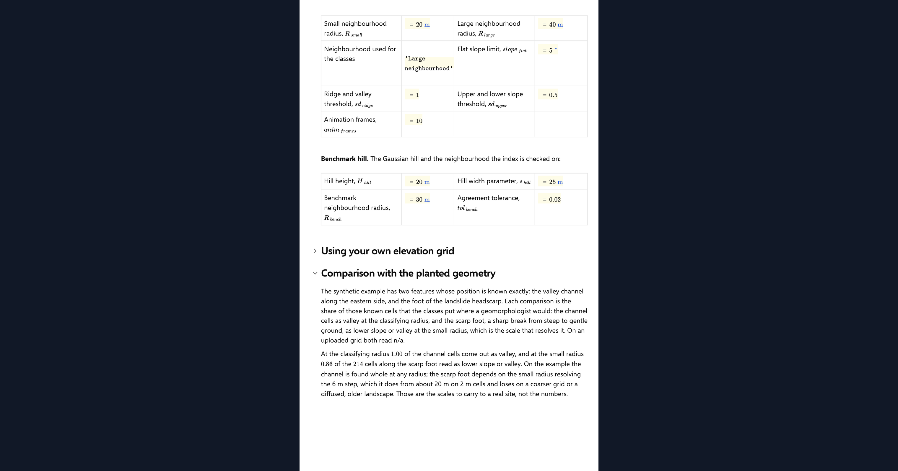
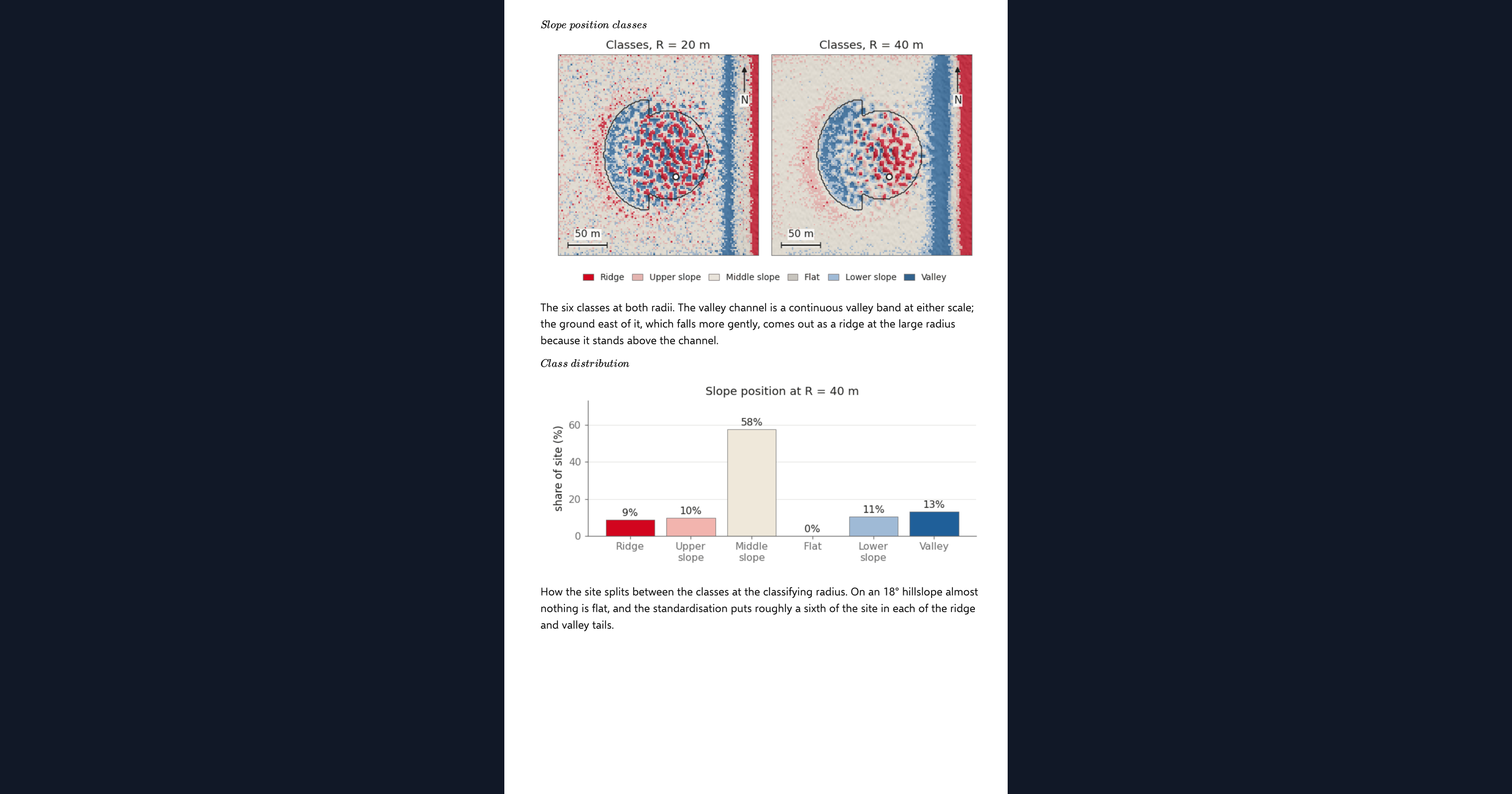
This page computes the topographic position index in Python, inside a CalcTree calculation page. Whether a point sits on a ridge, a slope or a valley floor is a question of where it stands relative to its surroundings, and the index answers it from an elevation grid alone. The page computes it at two neighbourhood radii, standardises it, classifies every cell into six slope positions (ridge, upper slope, middle slope, flat, lower slope and valley), maps the result over a hillshade and reads the class at a site you choose. It runs on a synthetic hillslope with a planted landslide and a valley, or on your own elevation grid uploaded as a CSV.

• Geotechnical engineer or engineering geologist: classify a site or a corridor by landform before a walkover, and see how the classes change between a local and a broad neighbourhood.
• Engineer exploring Python in calculations: read a landform classifier built from a disc mean, a plane fit and a few thresholds, with its benchmark, on one page.
• Graduate engineer learning terrain analysis: move the site, change the radii and the class thresholds and watch the map and the site class respond.

It is an analysis aid, not a site assessment. It is an example of what a CalcTree page can do, built with CalcTree AI, not a design method to rely on as is. The model is idealised and its limits are stated on the page. Duplicate it into your own workspace to change the inputs, read the Python, or use it as the starting point for your own analysis, and verify anything you take into a real design.

More info on the Topographic Position Index

Inputs

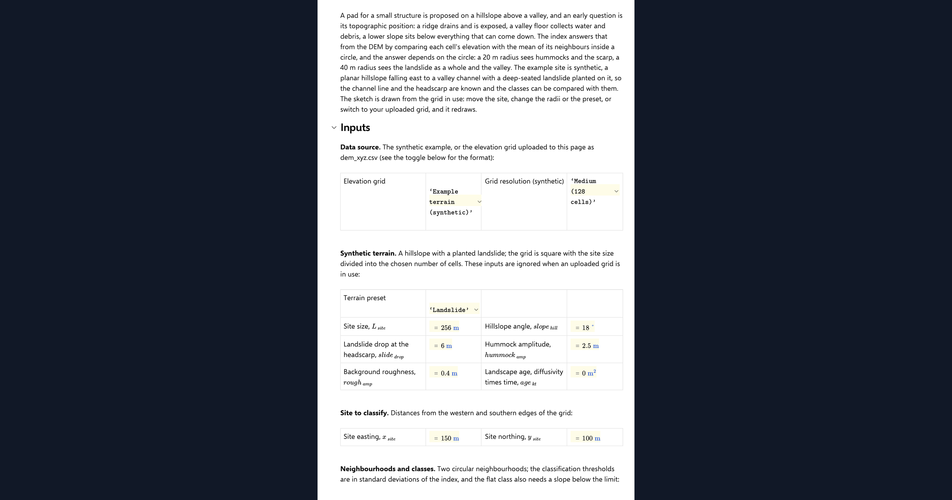
A data source dropdown chooses the example terrain or your uploaded grid. For the example you set a terrain preset, grid resolution, the planted landslide and its diffusion age. The method inputs are the site coordinates where the class is read, the small and large neighbourhood radii, which radius the classes are taken at, the thresholds in standard deviations that separate the classes, and the slope below which a near-zero index counts as flat. Your own elevation grid goes in as a CSV with x_m, y_m and z_m columns on a regular grid, loaded as a page dataset. The page refuses a grid that is not regular or is missing cells and says why, and it thins a grid wider than 192 cells a side to the smallest whole step that fits.

The index

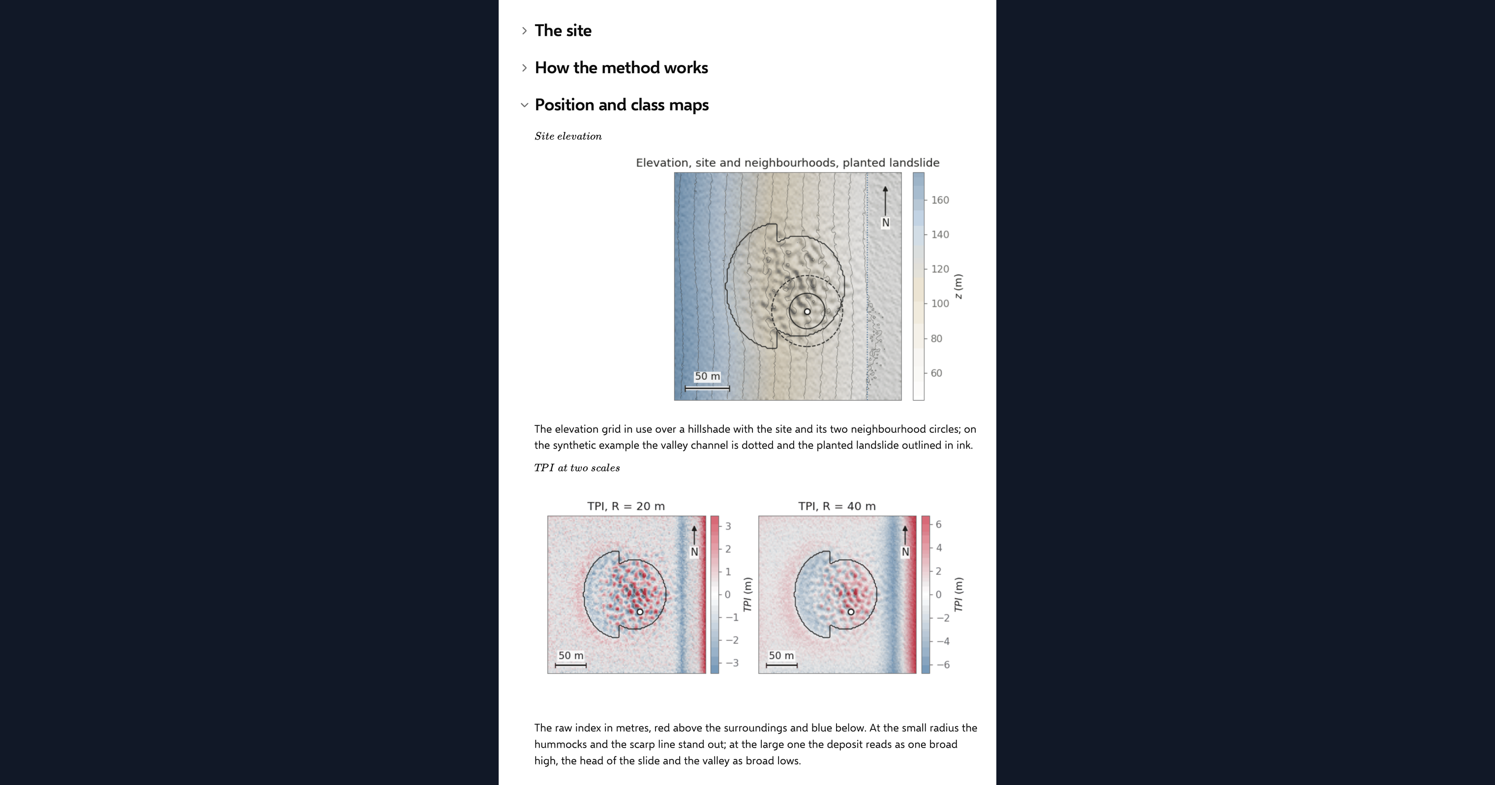
The topographic position index is the elevation of a cell minus the mean elevation of the cells within a disc around it, after Weiss (2001). A positive value is higher than its surroundings, a ridge or a crest; a negative value is a hollow or a valley; near zero is a uniform slope or a flat. The page evaluates the disc mean by convolution, on the residual from the grid's least-squares plane with symmetric padding, so a uniform hillslope reads zero everywhere including at the grid edges.

Two scales and six classes

The index depends on the radius. A small disc sees the hummocks and the scarp; a large one sees the whole hillside. The page computes both, standardises each over the grid, and classifies on the one you choose: ridge and valley beyond one standard deviation, upper and lower slope beyond half, and the band in between split into middle slope and flat by the local slope. The class shares and the class at your site are reported in the summary.

Checking the analysis

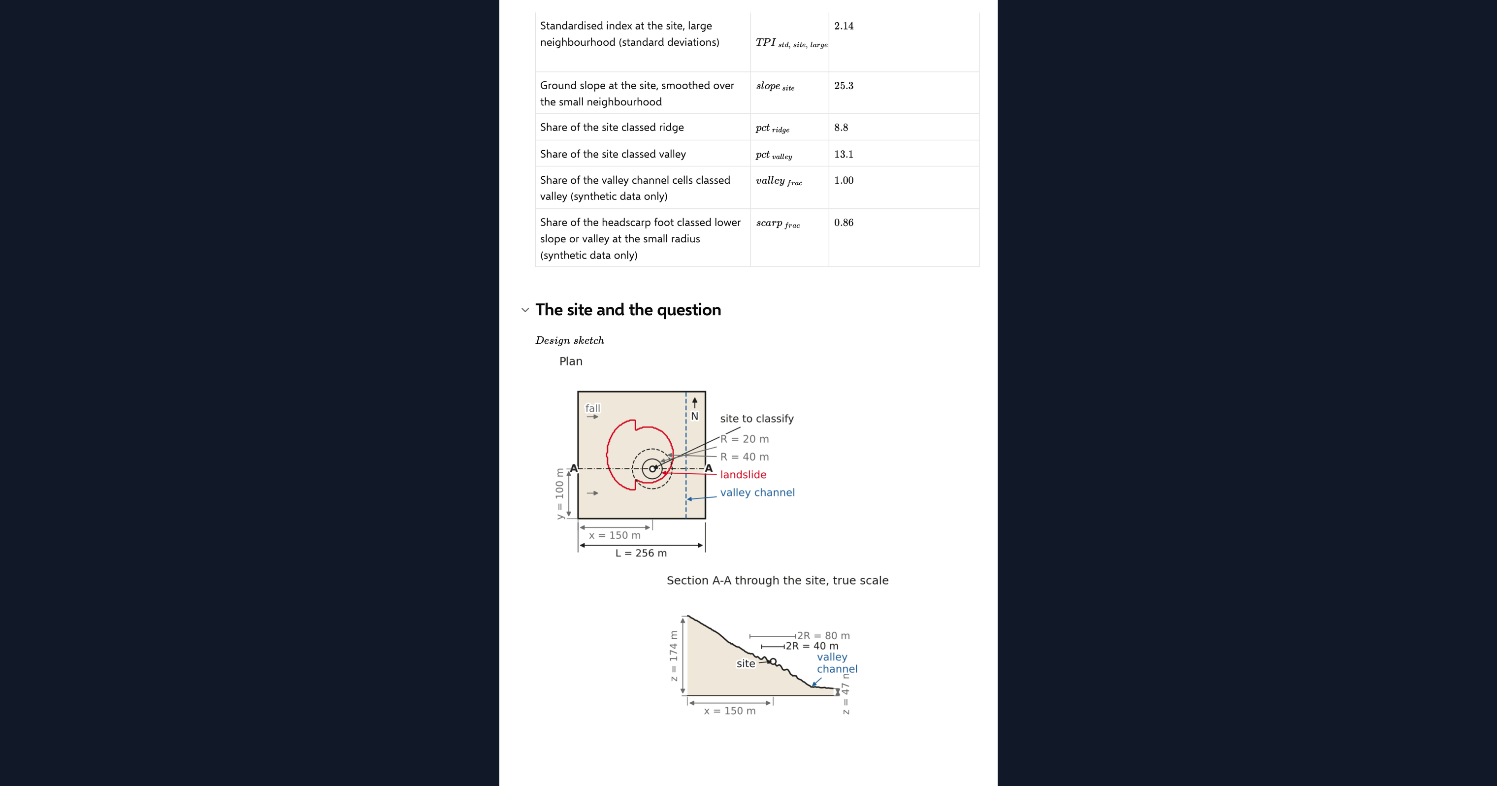
The index at the crest of a Gaussian hill has a closed form in the hill height, its width and the disc radius. The page builds that hill, evaluates its own index at the crest and compares the two in one agreement chip. On the example terrain it also reports how much of the known channel is classed valley and how much of the scarp foot is classed lower slope or valley, as results rather than verdicts.

Python libraries used

NumPy holds the grid and standardises the index. SciPy evaluates the disc mean by FFT convolution and the slope by filtered gradients. Matplotlib draws the hillshade, the index and class maps, the class distribution, the benchmark and the design sketch.

Common Calculation Errors to Avoid

• Reading a grid edge as a ridge: a plain disc mean on an inclined grid sees the uphill edge as high ground and the downhill edge as a valley. Detrend the grid and pad it symmetrically first.
• One radius for everything: a radius smaller than the landform cannot see it, and a radius larger than the grid flattens everything to a slope. Compute at least two and look at both.
• Standardising over the wrong area: the classes are set in standard deviations over the whole grid, so a grid that is mostly one big valley will put ordinary slopes in the ridge class. Keep the grid to the terrain you are classifying.
• Flat that is not flat: a near-zero index also occurs on a uniform steep slope. The flat class needs a slope test, which is why the page smooths the slope before applying it.
• Single-cell slope on noisy data: survey noise of a few tenths of a metre gives single-cell slopes of tens of degrees. Smooth over the small neighbourhood before using slope in a class rule.
• Treating the class as a hazard rating: a slope position says where a point stands, not whether it is stable. Use it to target investigation, not to replace it.

FAQs

What does a topographic position index value mean?

It is the height of a cell above or below the mean of its neighbourhood. Positive is a ridge or a crest, negative is a hollow or a valley, and near zero is either a flat or a uniform slope, which the local slope then separates.

Which neighbourhood radius should I use?

One that matches the landform you want to see. Tens of metres picks out scarps, hummocks and gullies; hundreds of metres picks out the hillside and the valley. The page computes two and lets you choose which to classify on, so compare them before settling.

Can I classify my own site?

Yes. Upload a regular x_m, y_m, z_m grid as the page dataset, switch the data source, and set the site coordinates. The class at the site, the class shares and the maps all come from your ground.

Why do the classes use standard deviations rather than metres?

So the same thresholds work on a gentle and a steep landscape. Standardising over the grid makes a ridge a feature that stands out from its own surroundings, which is the convention Weiss set and the one most published landform maps use.

How is the index checked?

Against a Gaussian hill, whose index at the crest has an exact expression in the hill height, its width and the disc radius. The page builds the hill, runs its own code on it and compares the two in one agreement chip.