
Free seismic time history example in Python: Newmark integration and response spectrum for a multi-storey frame. Open a copy in your browser.

Tell us what you need, or sign up and build it yourself in minutes.
Leave your email and we'll tell you when a template for it is ready:


No items found.
No items found.
About this Seismic Time History Example
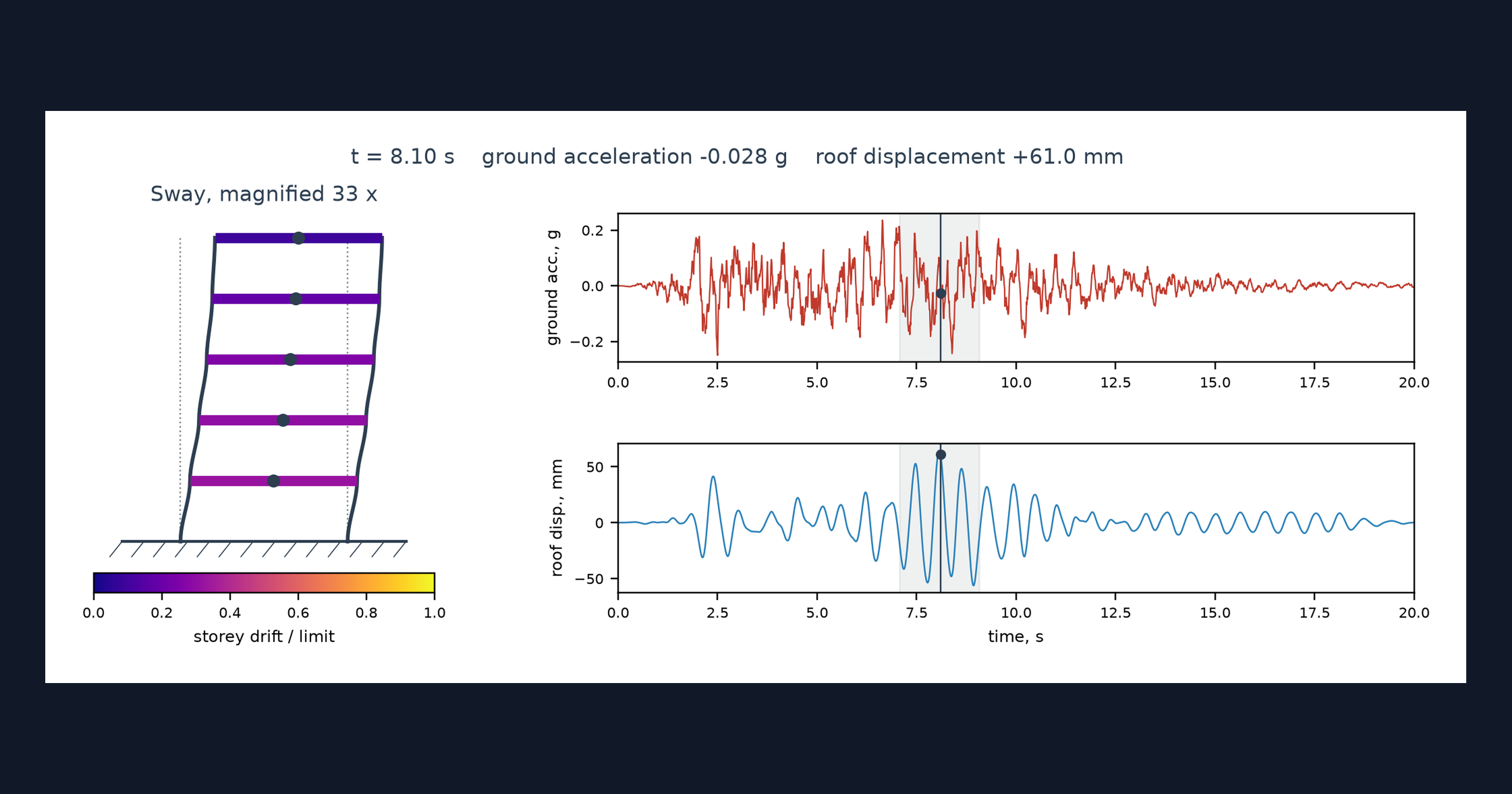
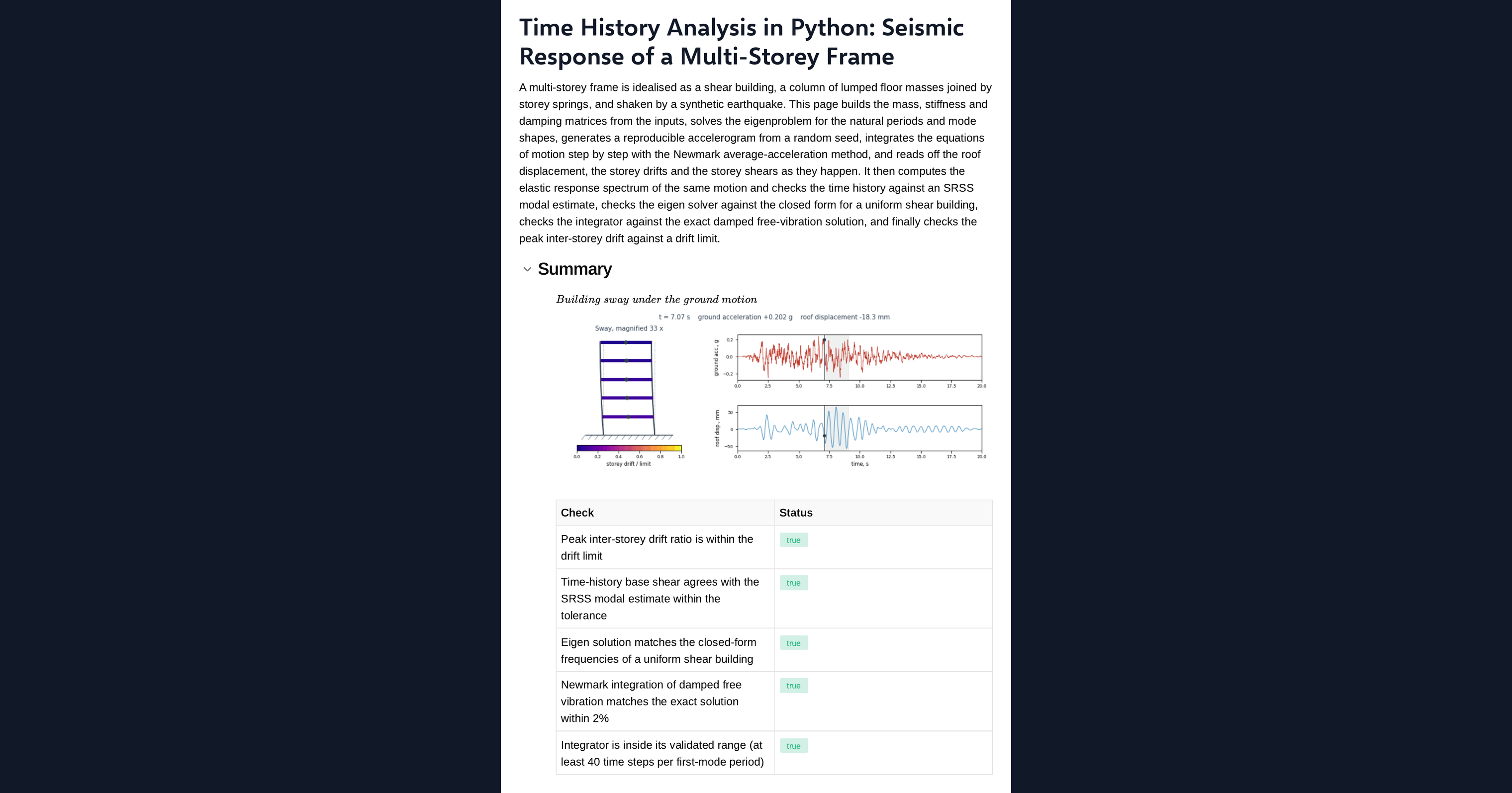
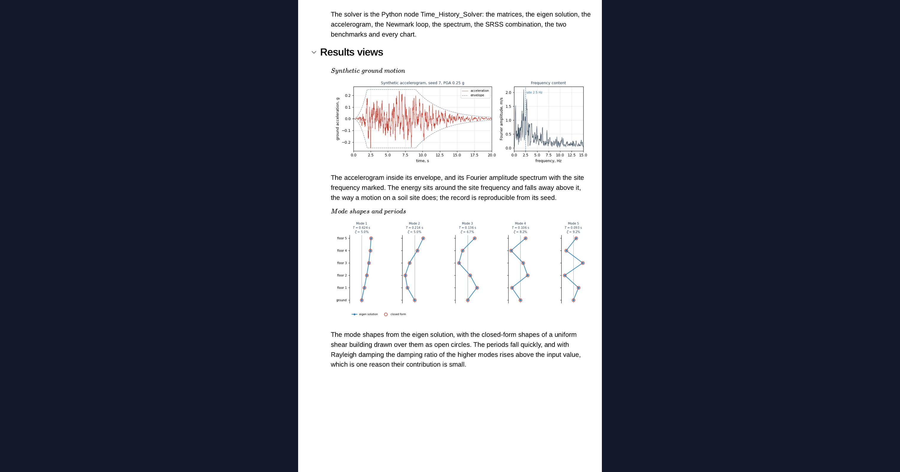
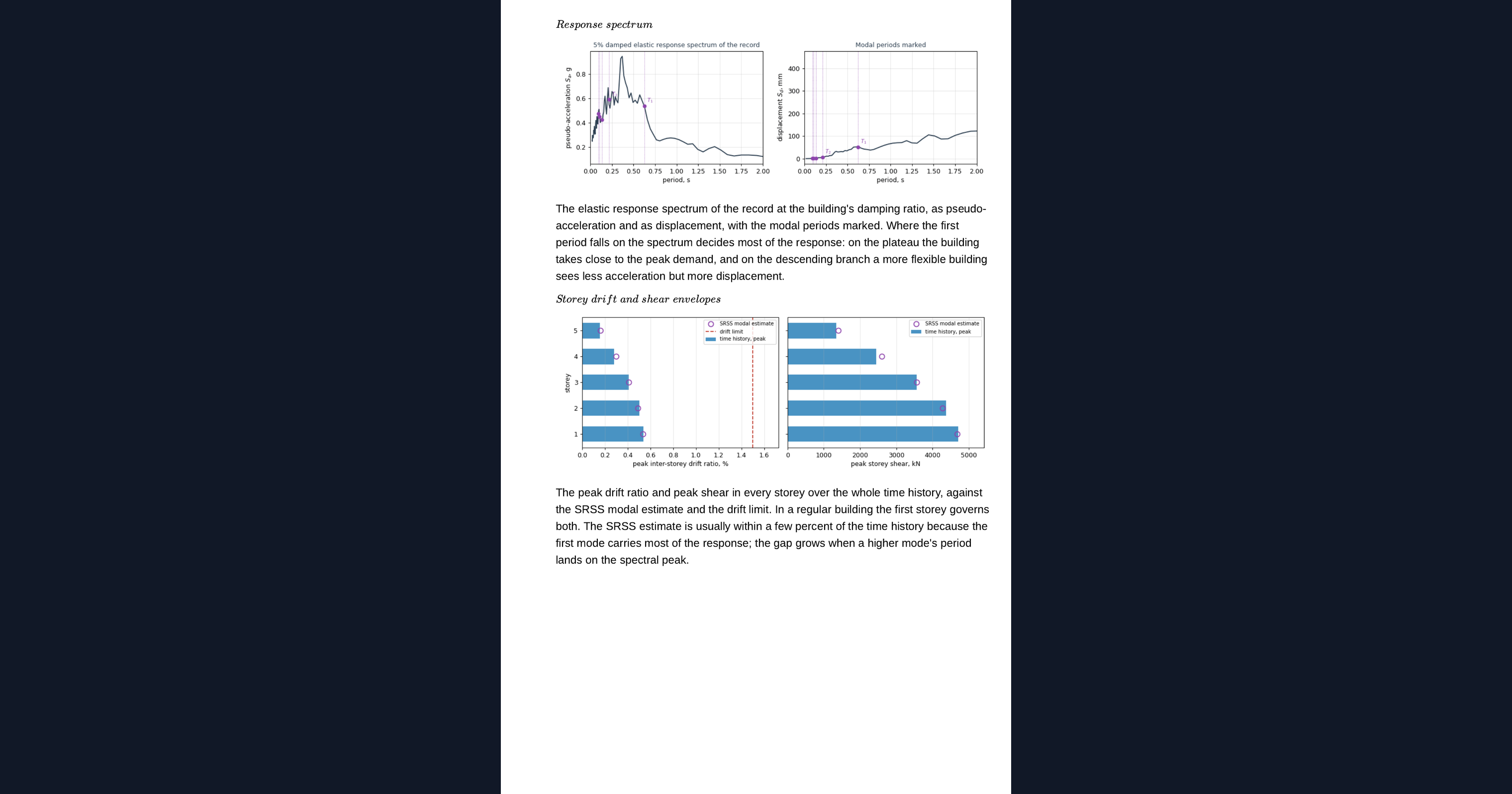
This page is a worked example of a seismic time history analysis in Python, running in your browser inside a CalcTree calculation page. It finds the modes of a multi-storey shear building, generates a synthetic ground motion, integrates the response with the Newmark method and animates the building swaying with the ground. From the same record it builds the response spectrum and compares the two methods, with the solver checked against closed-form results on the page.
- Structural engineer: see how a time history and a response spectrum of the same building compare, and adapt the example to your own frame.
- Earthquake engineering student: read a modal analysis, Newmark integrator and response spectrum in NumPy and SciPy, and watch the building sway.
- Engineer explaining seismic analysis: show a client or a team what a time history is, with the animation and the ground motion on one page.
It is an example of what a CalcTree page can do, built with CalcTree AI, not a design method to rely on as is. The model is idealised and its limits are stated on the page. Duplicate it into your own workspace to change the inputs, read the Python, or use it as the starting point for your own analysis, and verify anything you take into a real design.
More info on Seismic Time History Analysis
Inputs
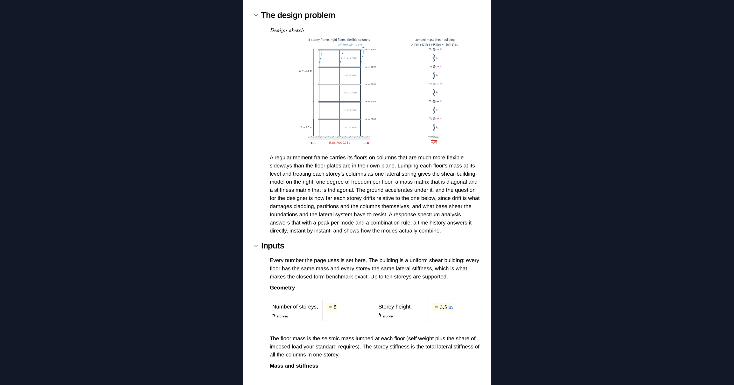
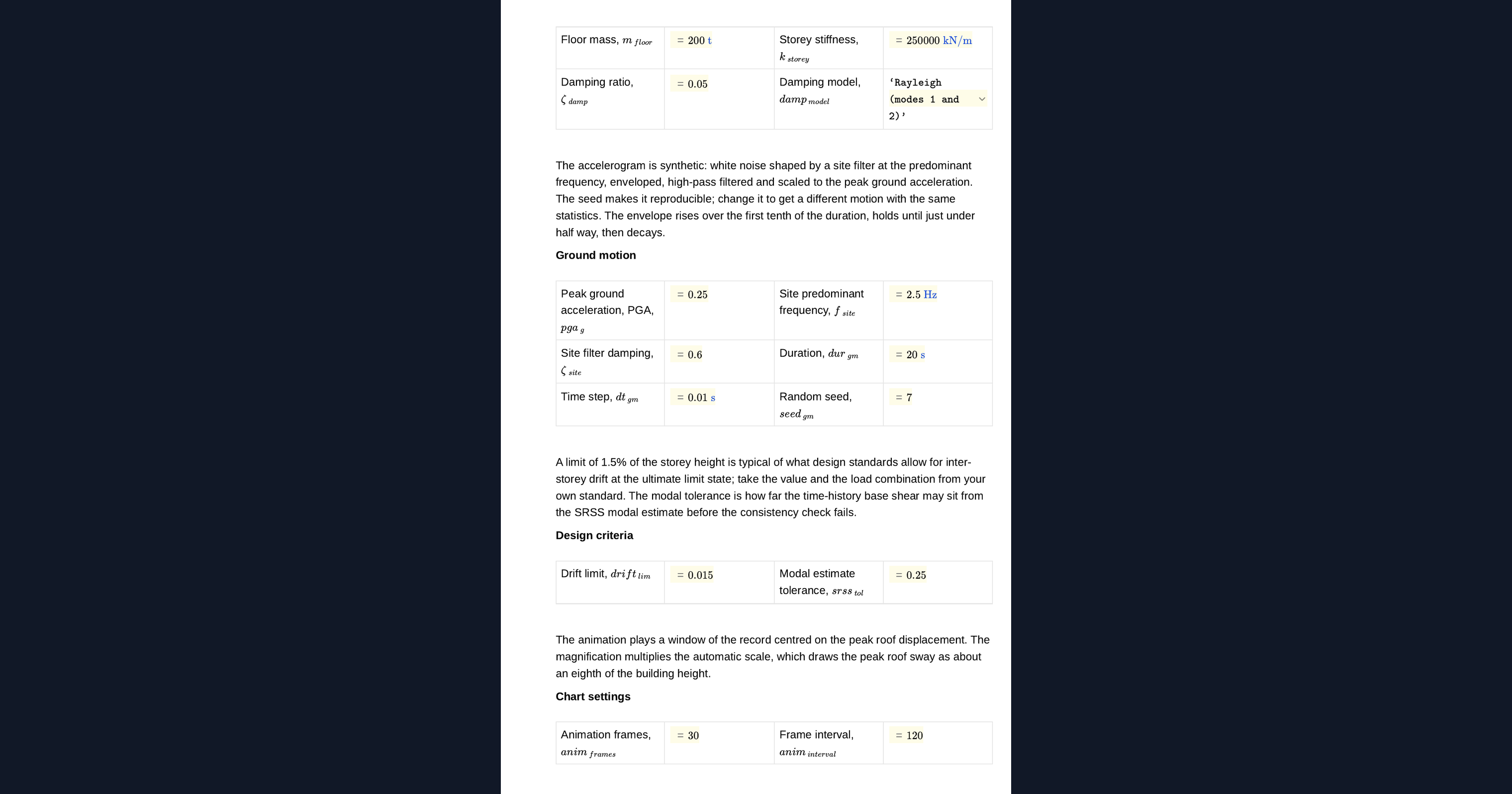
You set the number of storeys, the storey height, the floor mass and the storey stiffness, the damping ratio and the damping model. The ground motion is set by its peak ground acceleration, the site predominant frequency and filter damping, the duration, the time step and a random seed. The drift limit and the tolerance for the modal estimate are inputs too. A design sketch of the frame and its lumped-mass model redraws from them.
The time history method
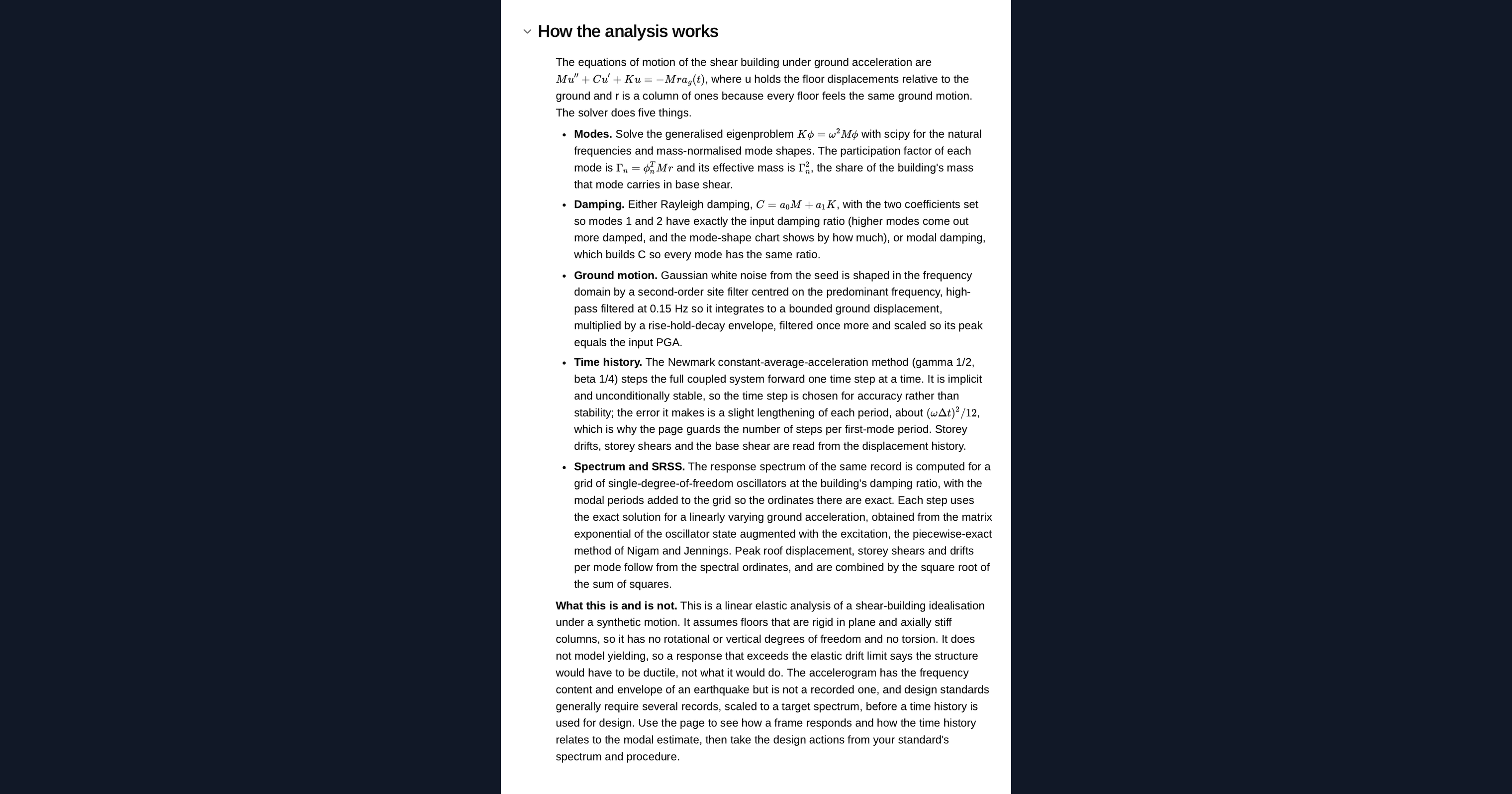
The building is a shear building: one mass per floor, connected by storey springs. The page solves the eigenvalue problem for its periods and mode shapes and builds a Rayleigh or modal damping matrix. The ground motion is white noise shaped by a site filter, wrapped in a rise, hold and decay envelope, and scaled to the peak ground acceleration. The Newmark average acceleration method then integrates the equations of motion through the record. The solver sits in a Python node on the page, so you can read it, change it and rerun it.
Checking the analysis
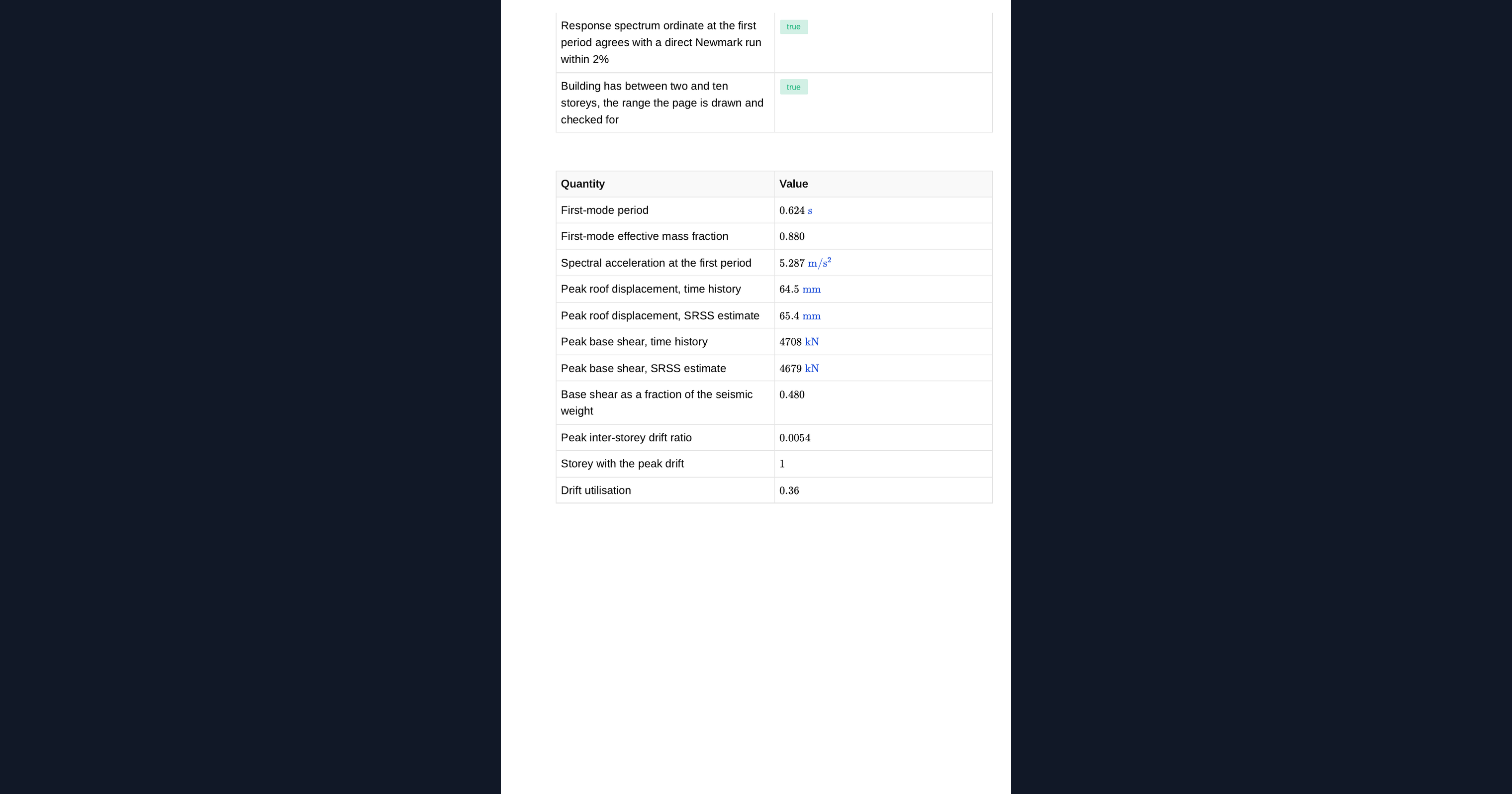
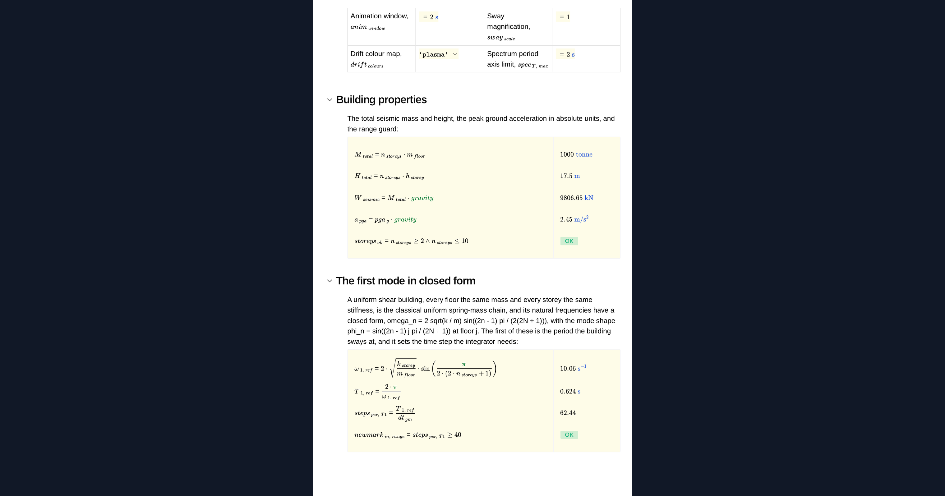
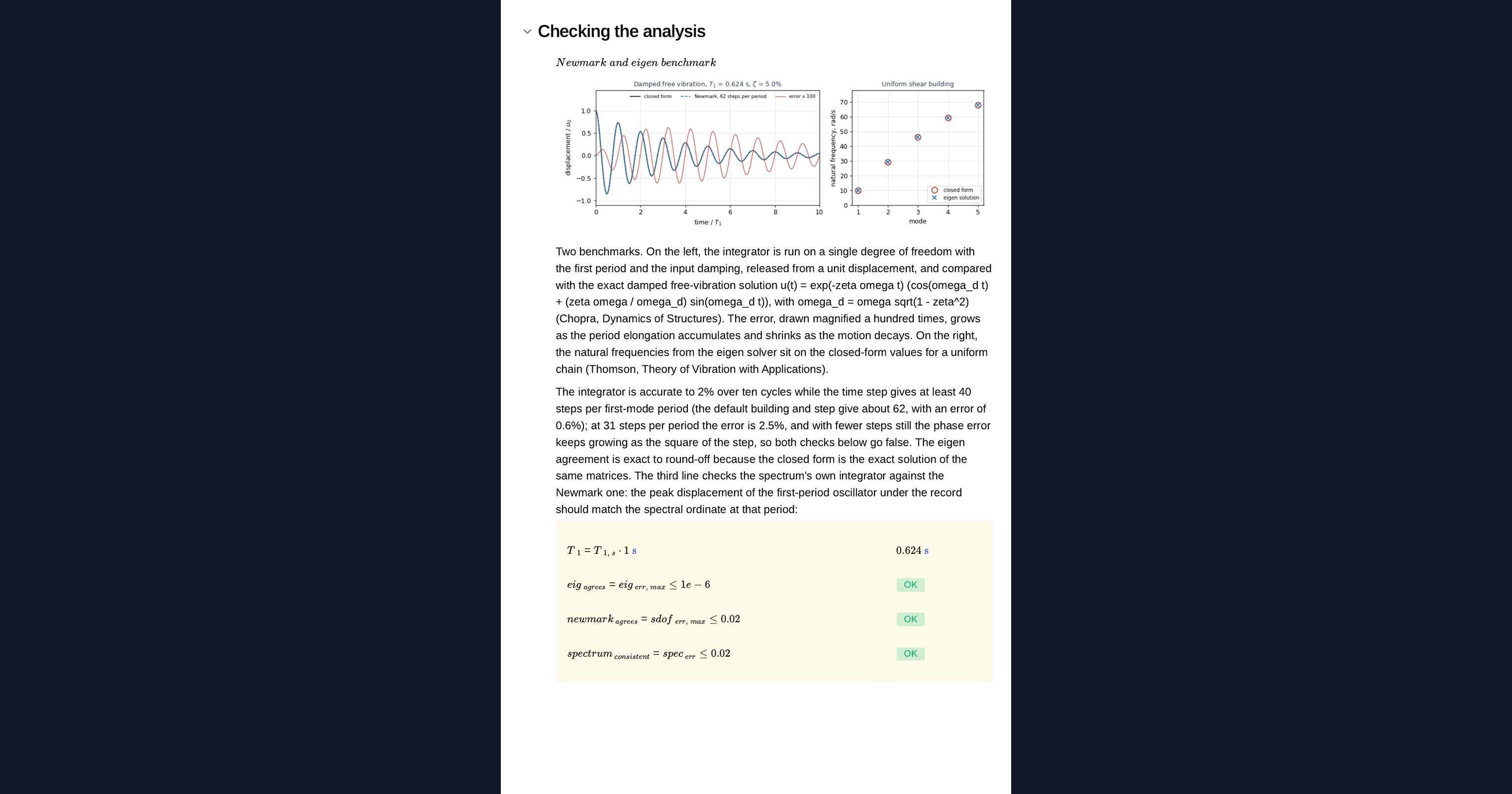
The periods are compared with the closed-form solution for a uniform spring-mass chain. The Newmark integrator is run on a single oscillator in free vibration and compared with the exact damped response. The response spectrum at the first period is compared with a direct single-oscillator run under the same record, and the modal combination of base shear with the time history. The page flags any result outside its tolerance, and whether the time step is fine enough for the first mode.
Drift and base shear
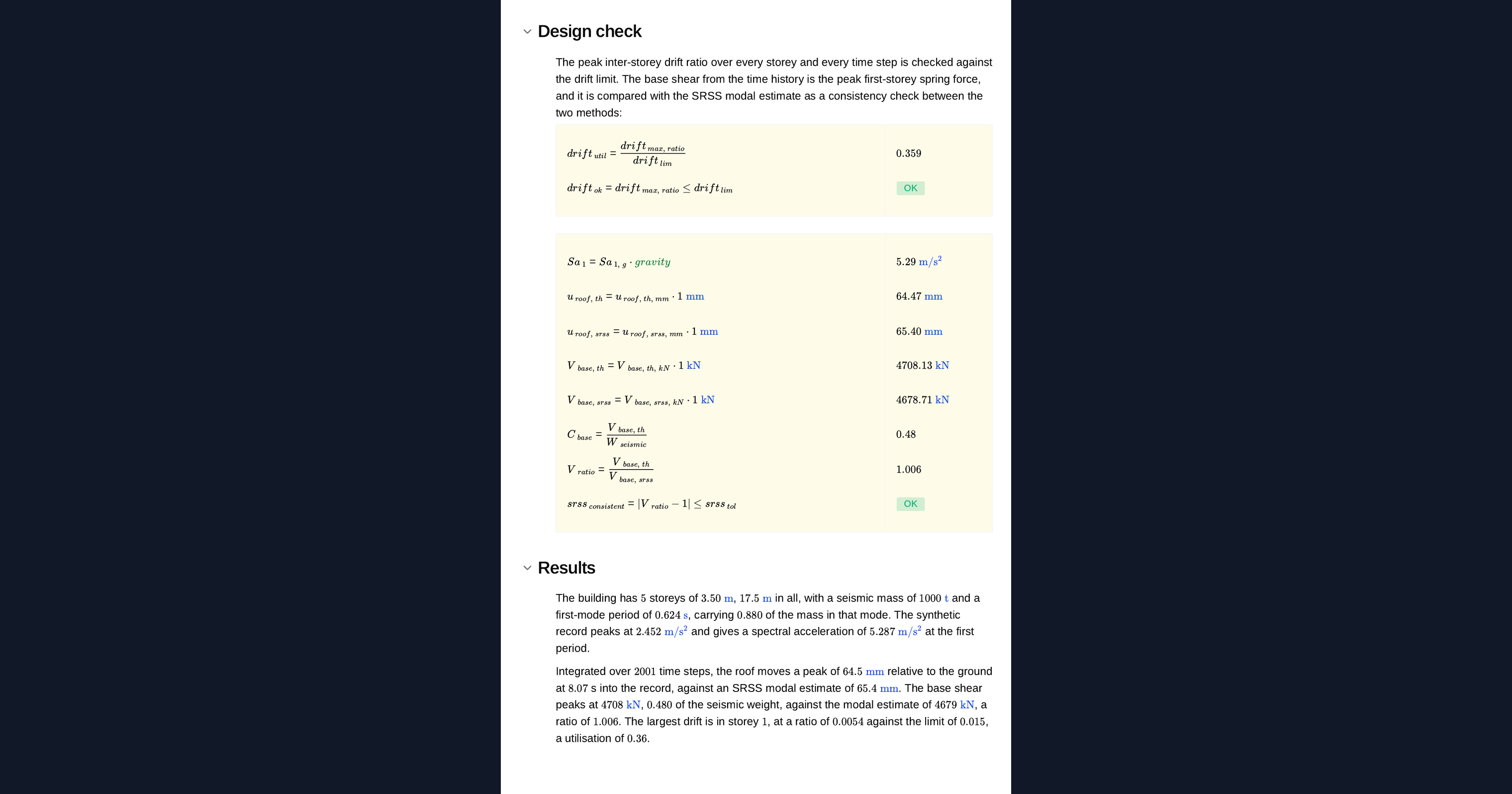
The page reports the roof displacement and base shear from both the time history and the modal combination, the base shear coefficient, and the peak interstorey drift ratio against the limit. It is a linear analysis under a single synthetic record, a demonstration of the method rather than a design to a standard, which generally needs several real records scaled to a target spectrum.
Python libraries used
NumPy builds the mass, stiffness and damping matrices, generates the ground motion and runs the Newmark integration. SciPy solves the eigenvalue problem for the modes and computes the matrix exponential behind the exact response spectrum step. Matplotlib draws the frame sketch, the ground motion, the response spectrum, the drift and shear envelopes and the animated building.
Common Calculation Errors to Avoid
- Designing to a single record: one ground motion is one sample, and codes generally require a suite of records scaled to the design spectrum.
- A time step too long for the first mode: the Newmark method lengthens the period as the step grows, so check the number of steps per period.
- Rayleigh damping on the higher modes: Rayleigh damping fixed on the first two modes over-damps the higher modes, which can understate their contribution.
- Treating a linear result as the real response: a linear model scales directly with the shaking and cannot show yielding, ductility or P-delta.
- Assuming the time history and the spectrum always agree: the combination rule is an estimate, and the two can differ noticeably for taller or more flexible buildings.
- Ignoring torsion and the real stiffness distribution: a shear building has uniform floors and no twist; real buildings need a full model.
Engineering templates
Common calculators
Design guides




FAQs
Can I run a seismic time history analysis in Python without ETABS or OpenSees?
For a linear shear building like this one, yes. The modes, the Newmark integration and the response spectrum fit in a short block of numpy and scipy, and this page checks each against a closed-form result. Use ETABS, SAP2000 or OpenSees for full three-dimensional models, nonlinear analysis and suites of real records.
What is the difference between time history and response spectrum analysis?
A time history steps the building through a ground motion and gives the full response over time. A response spectrum analysis takes only the peak response of each mode from a spectrum and combines them, which is quicker but an estimate. This page runs both on the same record so you can compare them.
What is the Newmark method?
A step-by-step method for integrating the equations of motion. The average acceleration version used here assumes the acceleration is constant over each step at the average of its start and end values, which is unconditionally stable and introduces no artificial damping.
Why does the page use a synthetic ground motion?
So the record is controlled by a few inputs and the page runs anywhere without a ground motion database. The page says plainly that a design time history needs several real records scaled to a target spectrum.
Can I change the building and rerun the analysis?
Yes. It is an example to build on: duplicate the page into your workspace, then change the building, the damping, the ground motion or the Python itself. The sketch, the animation, the spectrum and the checks all update together.
Learn about the benefits of using CalcTree on engineering projects!