Local, Distortional and Global Buckling Separated with pyCUFSM

Buckling modes, separated cleanly

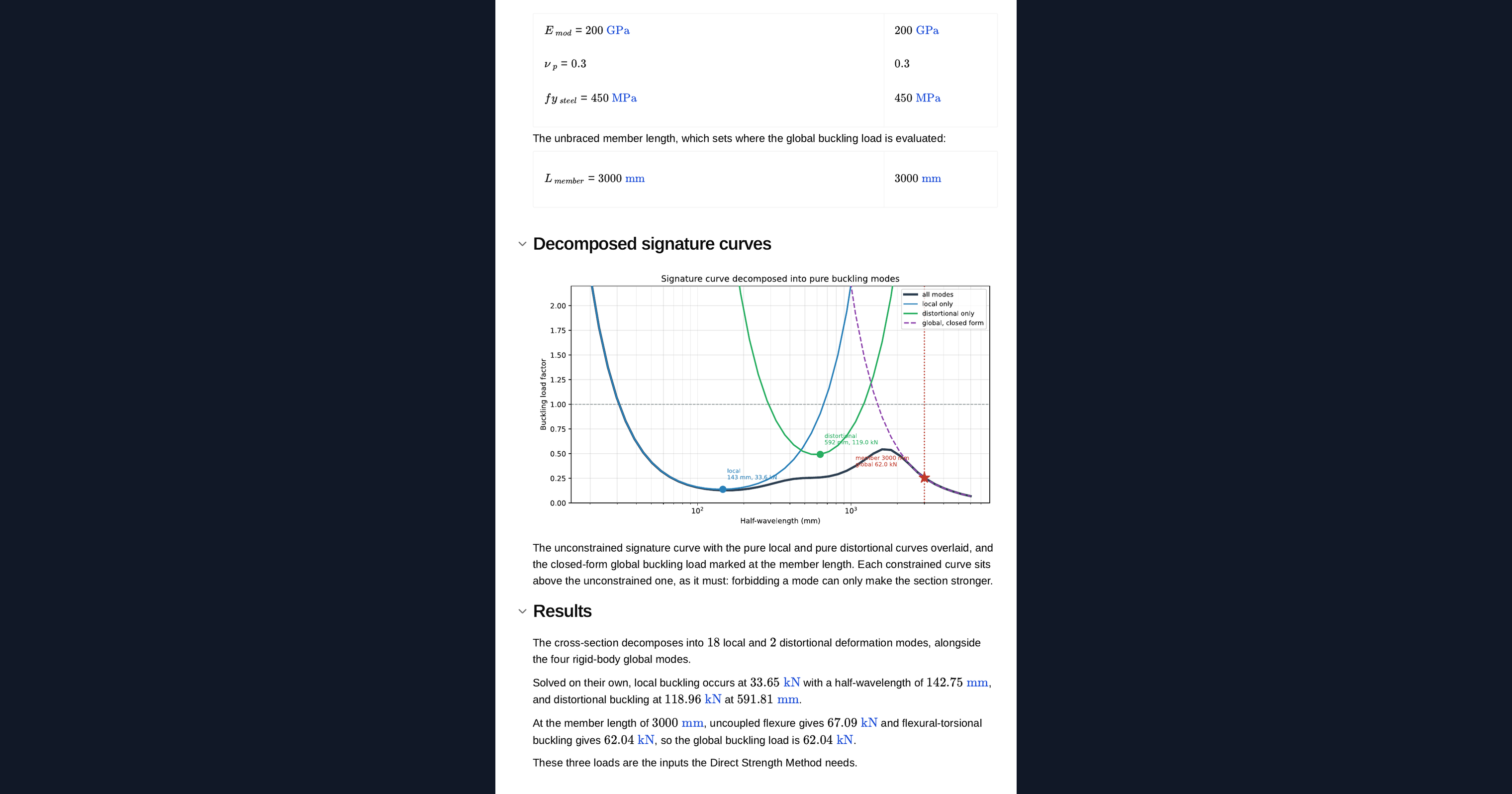
The signature curve of a cold-formed section mixes every buckling mode together. Where two modes sit close, the minimum of the curve does not cleanly belong to either, and one mode can hide behind another. This calculation uses constrained finite strip analysis to solve each mode family on its own, so the local, distortional and global buckling loads come out separately and unambiguously.

How it works

Ordinary finite strip analysis returns the lowest buckling load at each half-wavelength, whatever mode that happens to be. Usually the modes are well separated and the dips in the curve can be read off directly. Often they are not: a section with a short lip, or one carrying bending, can have local and distortional buckling at similar loads, and the single curve hides one behind the other.

Constrained finite strip analysis solves this by restricting the displacement field. The full space of cross-section deformations is decomposed into orthogonal sub-spaces, one for each mode family, according to the mechanics that define them:

• Global modes keep the cross-section undistorted. No plate bends and no fold line moves relative to another; the section translates and rotates as a rigid shape.
• Distortional modes allow the fold lines to move, but keep the plates straight in cross-section. The flange and lip rotate about the web-flange junction.
• Local modes hold every fold line fixed and let the plates bend between them. This is plate buckling of the individual flats.

Restricting the analysis to one sub-space returns the buckling load for that mode as if the others could not occur, which is exactly what the Direct Strength Method needs as input. The three curves are plotted together, so the interaction stays visible even though each load is computed in isolation.

Because the analysis runs a real finite strip solver (pyCUFSM) in the page, it handles arbitrary geometry entered as a table rather than a fixed standard case, and returns diagrams and contour plots alongside the numbers.

Limits and caveats

The decomposition assumes a single open branch with no closed cells. Sections with closed cells, or with branches meeting at a junction, need a different mode-space construction and are outside this template.

The global buckling load is computed in closed form, not by constrained strip analysis. The constrained global curve produced by the solver is not monotonic in half-wavelength: it reaches a minimum and then rises, which is physically impossible, since the load at which a member buckles as a rigid shape must fall as it gets longer. The unconstrained curve does not have this problem and reproduces the closed-form Euler load to within 0.3%, so the closed-form route is used instead and validated against it. This is also the conventional approach, because global buckling has to be evaluated at the member's real unbraced length rather than read off a half-wavelength axis.

Frequently asked questions

What is constrained finite strip analysis?

It is finite strip analysis in which the displacement field is restricted to a chosen sub-space of cross-section deformations. By decomposing the full deformation space into orthogonal families (global, distortional and local), each buckling mode can be solved on its own, rather than reading whichever mode happens to be lowest off a single signature curve.

Why not just read the modes off the signature curve?

When modes are well separated you can. But a short lip or a bending action can put local and distortional buckling at similar loads, and then the single curve shows only the lower of the two and hides the other. Solving each mode family separately removes that ambiguity.

How are the local, distortional and global modes defined?

Global modes keep the cross-section undistorted and let the member translate and rotate as a rigid shape. Distortional modes let the fold lines move while the plates stay straight in cross-section. Local modes hold the fold lines fixed and let the individual flats bend between them.

Why is global buckling computed in closed form instead of from the strip analysis?

The constrained global curve from the solver is not monotonic in half-wavelength: it dips and then rises, which cannot be right for a rigid-shape mode. The unconstrained curve reproduces the closed-form Euler load to within 0.3%, so the closed-form value is used and validated against it. Global buckling also has to be evaluated at the member's real unbraced length, not at a half-wavelength.

What sections can I analyse?

Any single open branch with no closed cells. Because the calculation runs a real finite strip solver on geometry you enter as a table, it is not limited to standard catalogue shapes. Sections with closed cells or branched junctions need a different mode-space construction and are not covered here.

How do the results feed the Direct Strength Method?

The Direct Strength Method needs the elastic local, distortional and global buckling loads as separate inputs. This calculation returns each one computed as if the others could not occur, which is precisely the form those inputs need to take.