
Fractal dimension of terrain in Python by the variogram method: map surface texture and outline the rough deposit, with a known-surface check. Open a copy.

Tell us what you need, or sign up and build it yourself in minutes.
Leave your email and we'll tell you when a template for it is ready:



No items found.
No items found.
About this Fractal Dimension Example
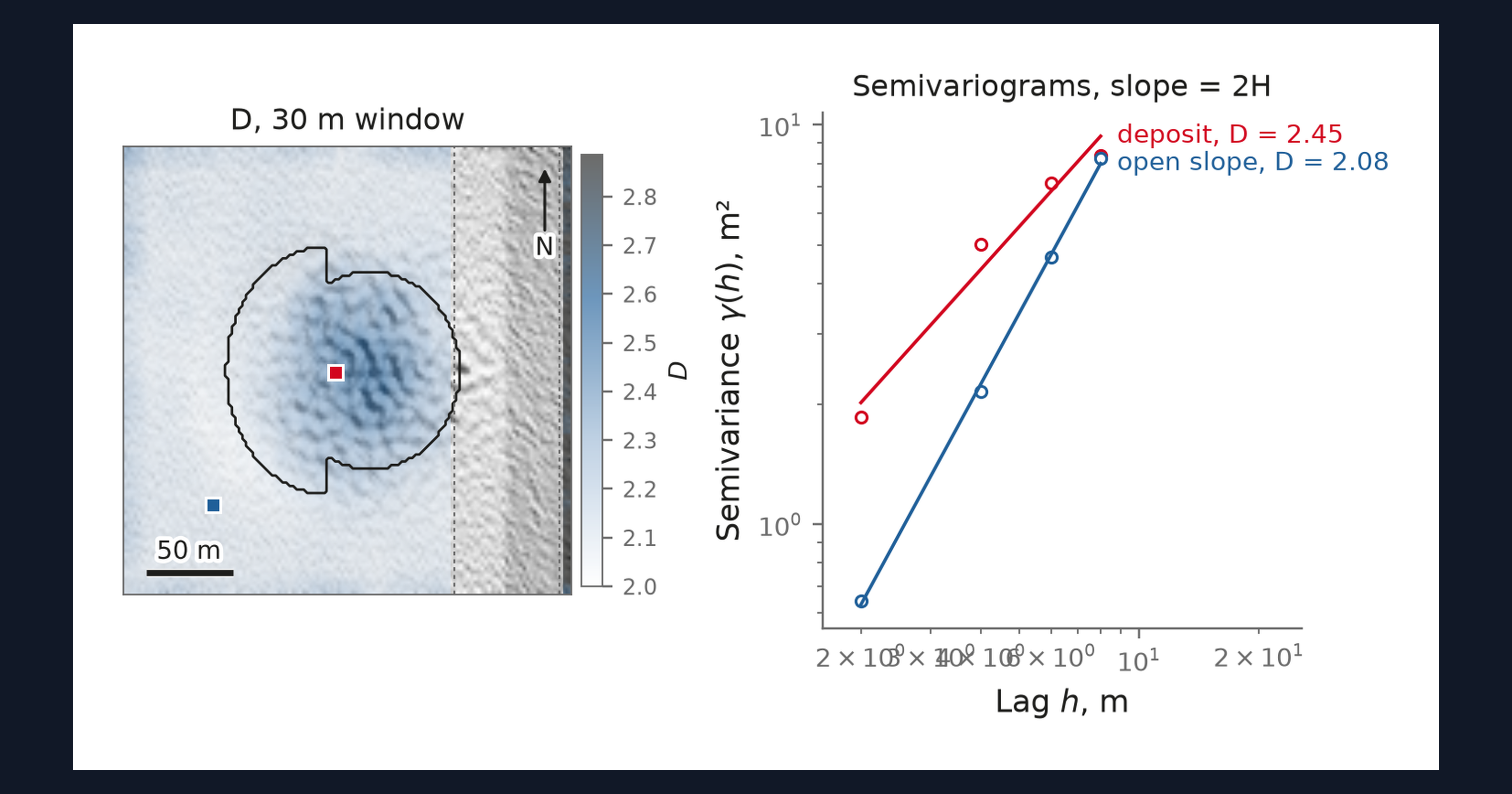
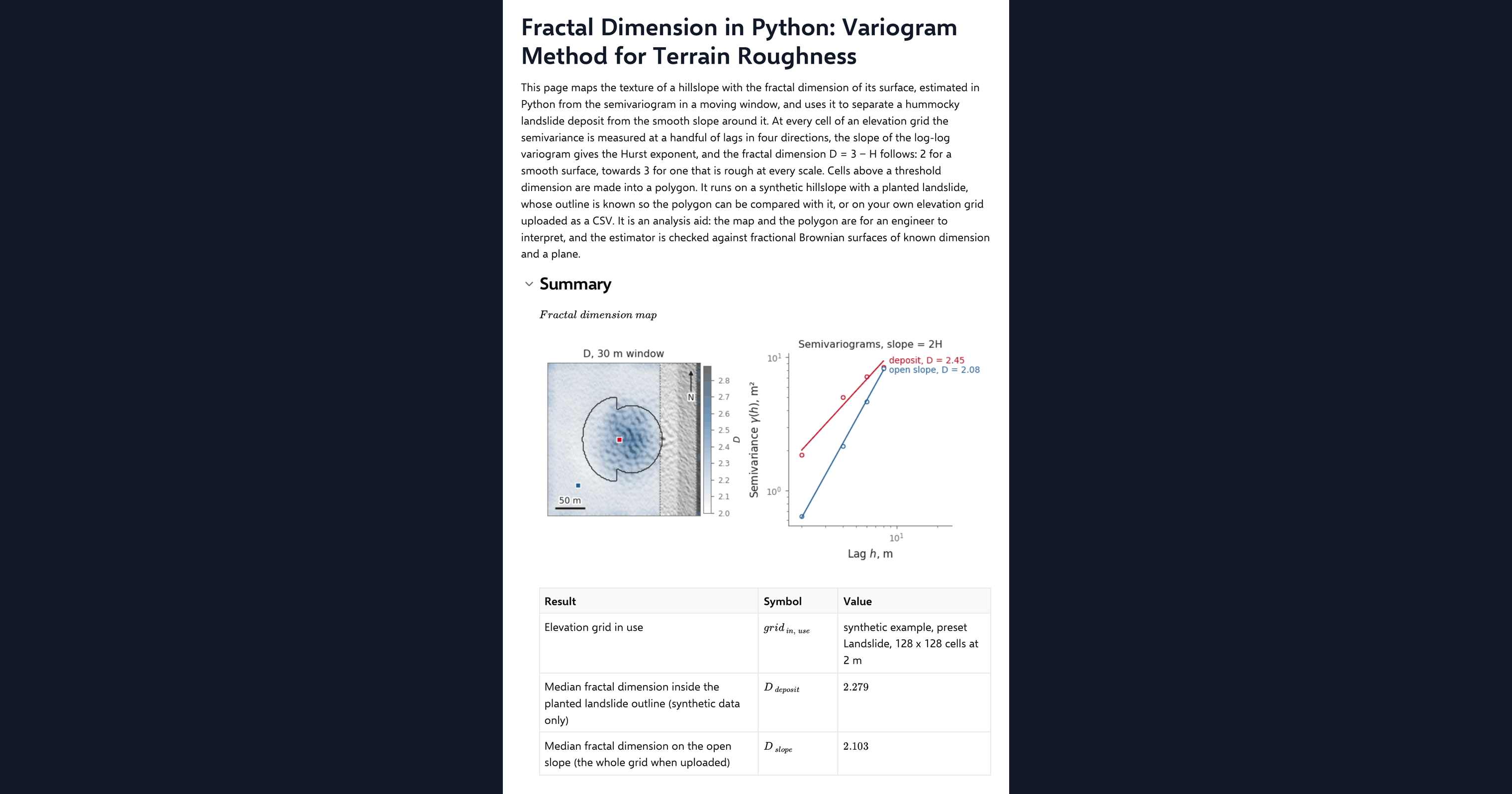
This page maps the fractal dimension of terrain in Python, inside a CalcTree calculation page. The dimension describes the texture of a surface: two for one that is smooth, towards three for one that is rough at every scale. At every cell of an elevation grid the page measures the semivariance at a handful of lags in four directions, takes the slope of the log-log variogram to get the Hurst exponent, and reports the dimension as three minus that exponent. Cells above a threshold dimension are made into a polygon, which on the synthetic hillslope can be compared with the planted landslide deposit. It also runs on your own elevation grid uploaded as a CSV.
- Engineering geologist or geotechnical engineer: separate a hummocky deposit from the smooth slope around it by texture rather than by height, and see how the lag range and window change what is mapped.
- Engineer exploring Python in calculations: read a variogram estimator, a fractal surface generator and a polygon clean-up in NumPy and SciPy on one page.
- Graduate engineer learning terrain analysis: change the window, the lags and the threshold and watch the map, the polygon and the benchmark respond.
It is an analysis aid, not a landslide assessment. It is an example of what a CalcTree page can do, built with CalcTree AI, not a design method to rely on as is. The model is idealised and its limits are stated on the page. Duplicate it into your own workspace to change the inputs, read the Python, or use it as the starting point for your own analysis, and verify anything you take into a real design.
More info on the Variogram Method
Inputs
A data source dropdown chooses the example terrain or your uploaded grid. For the example you set a terrain preset, grid resolution, the planted landslide and its diffusion age. The method inputs are the window the variogram is averaged over, the number of lags, the dimension threshold that defines rough ground, the width of the channel buffer excluded from the polygon, and the Hurst exponent of the synthetic surface used as a benchmark. Your own elevation grid goes in as a CSV with x_m, y_m and z_m columns on a regular grid, loaded as a page dataset. The page refuses a grid that is not regular or is missing cells and says why, and it thins a grid wider than 192 cells a side to the smallest whole step that fits.
The local variogram
The semivariance at a lag is half the mean squared difference in elevation between cells that distance apart. For a self-affine surface it grows as the lag to the power of twice the Hurst exponent, so the slope of the log-log variogram gives the exponent and the fractal dimension follows, after Mark and Aronson (1984) and Klinkenberg (1994). The page measures it in four lattice directions, averages it in a moving window with reflective padding, and fits the slope by least squares at every cell.
Mapping the deposit
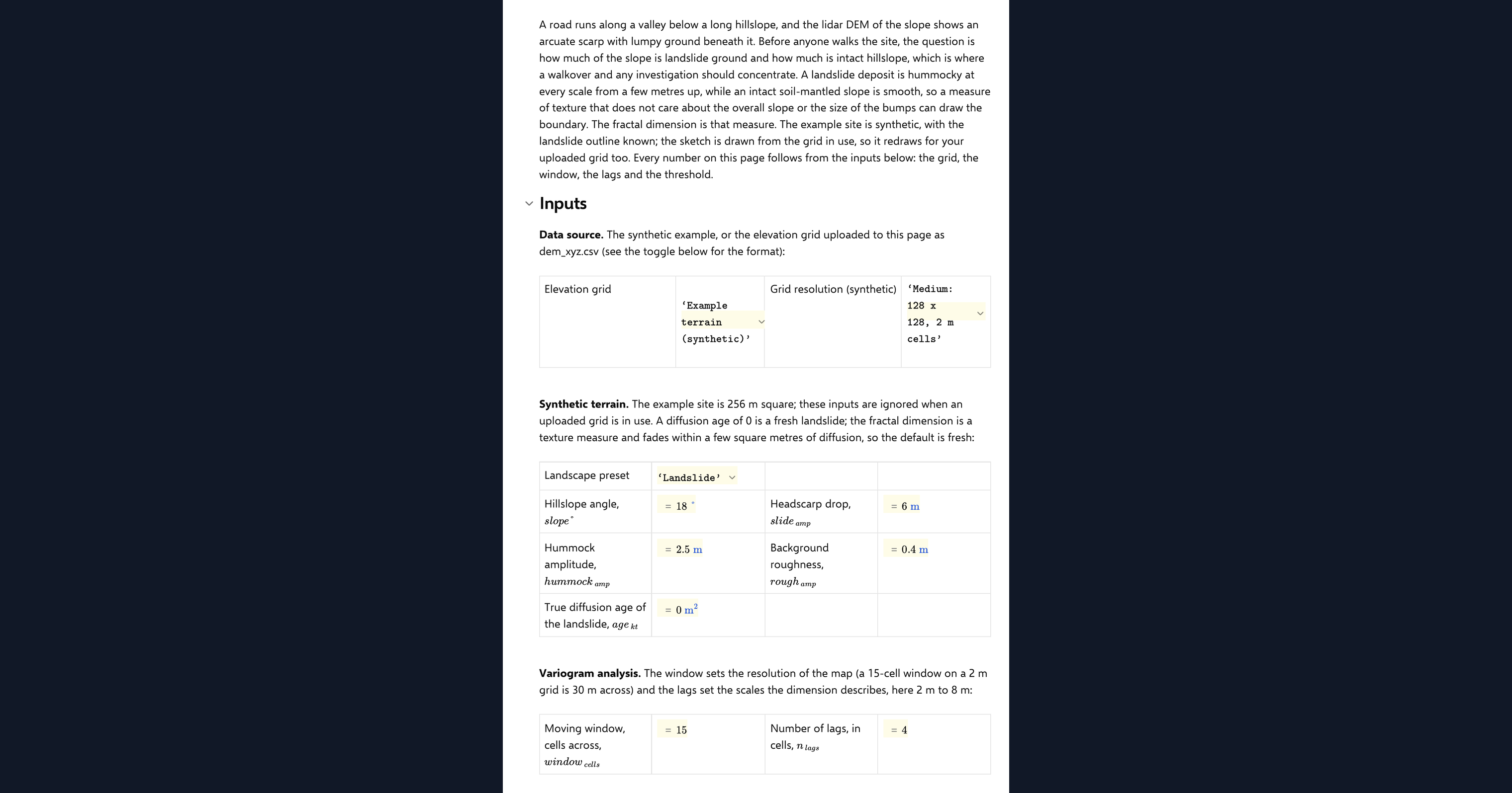
Cells above the threshold dimension, outside the channel buffer and clear of the window margin at the grid edge, are closed, hole-filled and eroded by the window radius to make a clean polygon. On the example terrain the overlap with the planted outline and the mapped area against the true area are reported as results. The deposit texture in the example is band-limited, so the contrast between deposit and slope is modest, and the page says so.
Checking the analysis
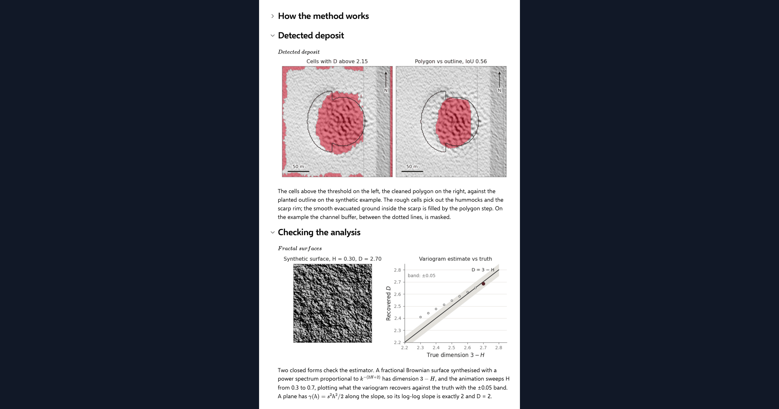
A fractional Brownian surface with a known Hurst exponent is synthesised in the spectral domain, and the page recovers its dimension by the same variogram code. The recovered value must sit within a stated tolerance of the known one for exponents in the range where the lattice estimator is unbiased, and a plane must return exactly two. One agreement chip reports both, with the range guard visible.
Python libraries used
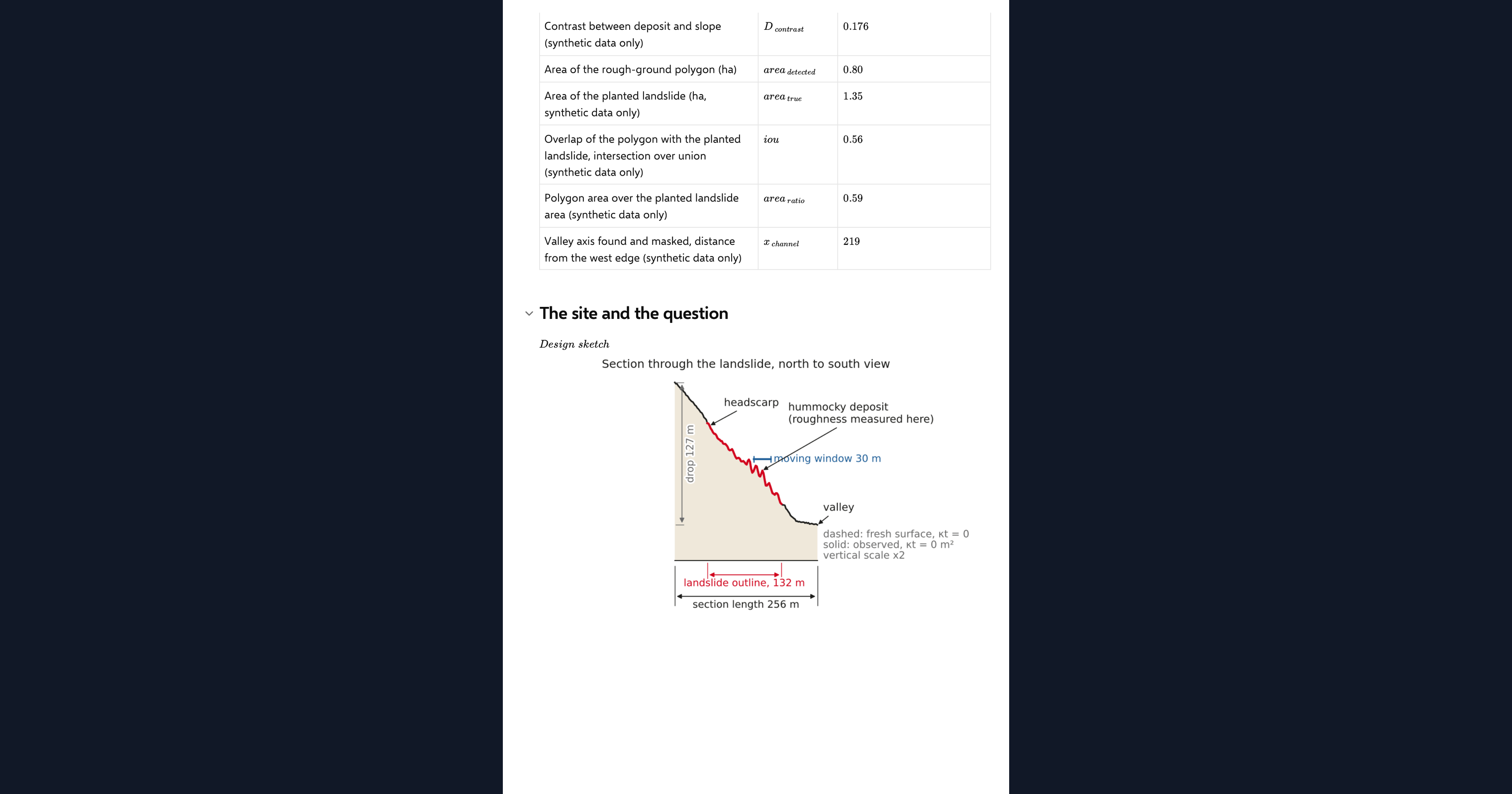
NumPy holds the grid, forms the lagged differences and fits the log-log slopes. SciPy averages the semivariance over the window and cleans the polygon with binary morphology. Matplotlib draws the hillshade, the dimension map, the mapped deposit, the fractal surfaces and the design sketch.
Common Calculation Errors to Avoid
- A lag range that spans the texture: lags longer than the hummock spacing make the variogram non-monotone and the fitted dimension collapses. Keep the lags shorter than the feature you want to see.
- Detrending before measuring: removing a plane first can make the survey noise the roughest thing in the grid and invert the contrast. The variogram of a plane is zero anyway, so measure the raw grid.
- Trusting the dimension at the grid edge: reflective padding anti-correlates the noise, and the dimension is inflated within half a window of the border. Exclude that margin from any polygon.
- Expecting an aged deposit to show: a few square metres of diffusion erases cell-scale texture and the dimension reads two everywhere. The method cannot date a deposit and does not see an old one.
- Fine grids and survey noise: on a finer grid the same noise is rougher per cell, so the slope's dimension rises and the polygon over-detects. Compare thresholds across resolutions before fixing one.
- Trusting the estimator at extreme exponents: the lattice variogram is biased at small lags for very smooth or very rough surfaces. The benchmark guards the range; stay inside it.
Engineering templates
Common calculators
Design guides




FAQs
What is the fractal dimension of a surface?
A measure of how rough it is across scales. A smooth surface has a dimension of two; one that stays rough however closely you look tends towards three. For terrain it sits between, and the difference between a smooth slope and a hummocky deposit is a few tenths.
How does the variogram give the dimension?
For a self-affine surface the semivariance grows as a power of the lag, and the exponent is twice the Hurst exponent. The slope of the log-log variogram gives that exponent, and the fractal dimension is three minus it. The page fits that slope in a moving window at every cell.
Why is the contrast between deposit and slope modest?
Because the example deposit is hummocky at one wavelength, and the dimension is a scale-free measure. Below that wavelength the hummocks look smooth, so the deposit reads only a few tenths above the slope. Real deposits with texture at many scales separate more clearly.
Can I run it on my own elevation grid?
Yes. Upload a regular x_m, y_m, z_m grid as the page dataset and switch the data source. The dimension map and the polygon then come from your ground, with no channel mask, and the comparison with a planted outline reads n/a.
How do I know the estimator is right?
The page synthesises a fractal surface with a Hurst exponent you set, recovers its dimension by the same code, and reports the error against a tolerance. A plane is also tested and must return exactly two.
Learn about the benefits of using CalcTree on engineering projects!